Chapter Eleven

Visual Thinking Processes

Many visualization systems are designed to help us hunt for new information, so different designs can be evaluated in terms of the efficiency with which knowledge can be gained. Pirolli and Card (1995) drew the following analogy between the way animals seek food and the way people seek information. Animals minimize energy expenditure to get the required gain in sustenance; humans minimize effort to get the necessary gain in information. Foraging for food has much in common with seeking information because, like edible plants in the wild, morsels of information are often grouped but separated by long distances in an information wasteland. Pirolli and Card elaborated the idea to include information “scent”—like the scent of food, this is the information in the current environment that will assist us in finding more succulent information clusters.

Reducing the cost of knowledge requires that we optimize cognitive algorithms that run on a peculiar kind of hybrid computer; part of this computer is a human brain, including its visual system, and part is a digital computer with a graphical display. In Chapter 1 we discussed user costs and benefits, but now we take a more system-oriented view with the following overarching principle for this chapter:

[G11.1] Design cognitive systems to maximize cognitive productivity.

Cognitive productivity is the amount of valuable cognitive work done per unit of time. Although it is only possible to put a value on this some of the time, maximizing productivity is nevertheless the (often implicit) goal of systems designed to support knowledge workers. In this chapter, we will be examining the characteristics of human–computer cognitive systems and the algorithms that run on them in order to better design systems that increase cognitive throughput.

The Cognitive System

An interactive visualization can be considered an internal interface between human and computer components in a problem-solving system. We are all becoming cognitive cyborgs in the sense that a person with a computer-aided design program, access to the Internet, and other software tools is capable of problem-solving strategies that would be impossible for that person acting unaided. A business consultant plotting projections based on a spreadsheet business model can combine business knowledge with the computational power of the spreadsheet to plot scenarios rapidly, interpret trends visually, and make better decisions.

Figure 11.1 illustrates the key components of this kind of cognitive system. On the human side, a critical component is visual working memory; we will be concerned especially with the constraints imposed by its low capacity. At any given instant, visual working memory contains a small amount of information relating to the visual display generated by a computer. It can also contain information about the visual query that is being executed by means of a visual pattern search.

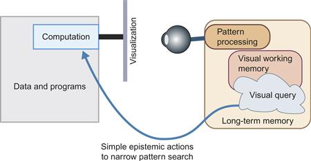
Figure 11.1 The cognitive system considered in this chapter.

For visual queries to be useful, a problem must first be cast in the form of a visual pattern that, if identified, helps solve part of the problem. Finding a number of big red circles in a geographic information system (GIS) display, for example, may indicate a problem with water pollution. Finding a long, red, fairly straight line on a map can show the best way to drive between two cities. Once the visual query is constructed, a visual pattern search provides answers.

Part of the thinking process consists of what Karsh (2009) calls epistemic actions. These can be eye movements to pick up more information. Or, in the case of an interactive visualization, these can be mouse movements, causing programs to execute in the computer, changing the nature of the information that is displayed. These computer-side operations, such as brushing to highlight related information or zooming in on some information, make it easier to process visual queries by finding task-relevant patterns. Alternatively, the selection of a visual object may trigger the highlighting of other objects that a computer algorithm suggests are relevant. This narrows the visual search, speeding the resolution of a visual query. We will focus here mostly on tight loop interactions, where human actions trigger relatively simple and rapid transformations of what is presented on a display.

Another important role of visualizations is as a form of memory extension. This comes about from the way a displayed symbol, image, or pattern can rapidly evoke nonvisual information and cause it to be loaded from long-term memory into verbal/propositional processing centers.

The most important contribution of this chapter is a set of visual thinking algorithms. These are processes executed partly in the brain of a person and partly in a computer, but there is an essential component of visual perception that we need to describe first. We have so far neglected visual memory and its relationship to nonvisual memory as well as attention, and how these processes are critical to understanding visual thinking; therefore, the first third of this chapter is devoted to memory systems, following which the algorithms are described.

Memory and Attention

As a first approximation, there are three types of memory: iconic, working, and long-term (see Figure 11.2). There may also be a fourth, intermediate store that determines which information from working memory finds its way into long-term memory.

Figure 11.2 Three types of memories are iconic stores, working memory stores, and long-term memory stores.

Iconic memory is a very short-term image store, holding what is on the retina until it is replaced by something else or until several hundred milliseconds have passed (Sperling, 1960). This is image-related information, lacking semantic content.

Visual working memory holds the visual objects of immediate attention. The contents of working memory can be drawn from either long-term memory (in the case of mental images) or input from the eye, but most of the time information in working memory is a combination of external visual information made meaningful through the experiences stored in long-term memory.

Long-term memory is the information that we retain from everyday experience, perhaps for a lifetime, but it should not be considered as separate from working memory. Instead, working memory can be better conceived of as information activated within long-term memory.

Of the three different stores, working memory capacities and limitations are most critical to the visual thinking process.

Working Memories

There are separate working memory subsystems for processing auditory and visual information, as well as subsystems for body movements and verbal output (Thomas et al., 1999). There may be additional working memory stores for sequences of cognitive instructions and for motor control of the body. Kieras and Meyer (1997), for example, proposed an amodal control memory containing the operations required to accomplish current goals and a general-purpose working memory containing other miscellaneous information. A similar control structure is called the central executive in Baddeley and Hitch’s (1974) model. A more modern view is that there is no central processor; instead, different potential activation loops compete with a winner-take-all mechanism, causing only one to become active. This determines what we will do next (Carter et al., 2011).

Visual thinking is only partly executed using the uniquely visual centers of the brain. In fact, it emerges from the interplay of visual and nonvisual systems, but because our subject is visual thinking we will hereafter refer to most nonvisual processes generically as verbal–propositional processing (see Chapter 9 for a discussion of the issues relating to representations based on words and images). It is functionally quite easy to separate visual and verbal–propositional processing. Verbal–propositional subsystems are occupied when we speak, whereas visual subsystems are not. This allows for simple experiments to separate the two processes. Postma and De Haan (1996) provided a good example. They asked subjects to remember the locations of a set of easily recognizable objects—small pictures of cats, horses, cups, chairs, tables, etc.—laid out in two dimensions on a screen. The objects were then placed in a line at the top of the display and the subjects were asked to reposition them in their original locations, a task the subjects performed quite well. In another condition, subjects were asked to repeat a nonsense syllable, such as “blah,” while in the learning phase. This time, they did much worse. Saying “blah” did not disrupt memory for the locations themselves; instead, it only disrupted memory for what was at the locations. This was demonstrated by having subjects place a set of disks at the positions of the original objects, which they could do with relative accuracy. In other words, when “blah” was said in the learning phase, subjects learned a set of locations but not the objects at those locations. This technique is called articulatory suppression. The reason why saying “blah” disrupted working memory for the objects is that task-relevant object information was stored using a verbal–propositional coding. The reason it did not disrupt location information is because place information was held in visual working memory.

Visual Working Memory Capacity

Visual working memory can be roughly defined as the visual information retained from one fixation to the next. Position is not the only information stored in visual working memory; some abstract shape, color, and texture information is also retained. This appears to be limited to about three to five simple objects (Irwin, 1992; Luck & Vogel, 1997; Melcher, 2001; Xu, 2002). The exact number depends on the task and the kind of pattern.

Figure 11.3(a) illustrates the kinds of patterns used in a series of experiments by Vogel et al. (2001) to study the capacity of visual working memory. In these experiments, one set of objects was shown for a fraction of a second (e.g., 0.4 sec), followed by a blank of more than 0.5 sec. After the blank, the same pattern was shown, but with one attribute of an object altered—for example, its color or shape. The results from this and a large number of similar studies have shown that about three objects can be retained without error, but these objects can have color, shape, and texture. If the same amount of color, shape, and texture information is distributed across more objects, memory declines for each of the attributes.

Figure 11.3 Patterns used in studies of the capacity of visual working memory. (a, c) From Vogel et al. (2001). (b) From Xu (2002). Reproduced with permission.

Only quite simple shapes can be stored in this way. Each of the mushroom shapes shown in Figure 11.3(b) uses up two visual memory slots (Xu, 2002). Subjects do no better if the stem and the cap are combined than if they are separated. Intriguingly, Vogel et al. (2001) found that if colors were combined with concentric squares, as shown in Figure 11.3(c), then six colors could be held in visual working memory, but if they were put in side-by-side squares, then only three colors could be retained. Melcher (2001) found that more information could be retained if longer viewing was permitted, up to five objects after a 4-sec presentation.

What are the implications for data glyph design? (A glyph, as discussed in Chapter 5, is a visual object that displays one or more data variables.) If it is important that a data glyph be held in visual working memory, then it is important that its shape allows it to be encoded according to visual working memory capacity. Figure 11.4 shows two ways of representing the same data. One consists of an integrated glyph containing a colored arrow showing orientation by arrow direction, temperature by arrow color, and pressure by arrow width. A second representation distributes the three quantities among three separate visual objects: orientation by an arrow, temperature by the color of a circle, and air pressure by the height of a rectangle. The theory of visual working memory and the results of Vogel et al. (2001) suggest that three of the integrated glyphs could be held in visual working memory, but only one of the nonintegrated glyphs.

Figure 11.4 If multiple data attributes are integrated into a single glyph, more information can be held in visual working memory.

Change Blindness

The finding that visual working memory has a very low capacity has extraordinary implications for how we see and what we see in general, as well as how we interpret visualizations. Among other things it suggests that our impression that we see the world in all its complexity and detail is illusory. In this section, we review some of the evidence showing that this is in fact the case.

One of the consequences of the very small amount of information held in visual working memory is a phenomenon known as change blindness (Rensink, 2000). Because we remember so little, it is possible to make large changes in a display between one view and the next, and people generally will not notice unless the change is to something they have recently attended. If a change is made while the display is being fixated, the rapid visual transition will draw attention to it. But, if changes are made mid-eye movement, mid-blink, or after a short blanking of the screen (Rensink, 2002), then the change generally will not be seen. Iconic memory information in retinal coordinates decays within about 200 msec (Phillips, 1974). By the time 400 msec have elapsed, what little remains is in visual working memory.

An extraordinary example of change blindness is a failure to detect a change from one person to another in mid-conversation. Simons and Levin (1998) carried out a study in which an unsuspecting person was approached by a stranger holding a map and asking for directions. The conversation that ensued was interrupted by two workers carrying a door and during this interval another actor, wearing different clothes, was substituted to carry on the conversation. Remarkably, most people did not notice the substitution.

To many people, the extreme limitation on the capacity of visual working memory seems quite incredible. How can we experience a rich and detailed world, given such a shallow internal representation? Part of the answer to this dilemma is that the world “is its own memory” (O’Regan, 1992). We perceive the world to be rich and detailed, not because we have an internal detailed model, but simply because whenever we wish to see detail we can get it, either by focusing attention on some aspect of the visual image at the current fixation or by moving our eyes to see the detail in some other part of the visual field. We are unaware of the jerky eye movements by which we explore the world and only aware of the complexity of the environment through detail being brought into working memory on a need-to-know, just-in-time fashion (O’Regan, 1992; Rensink et al., 1997; Rensink, 2002).

A second part of the explanation of how we sustain the illusion of seeing a rich and detailed word is gist. Gist is the activated general knowledge we have about particular kinds of environments. Much of the information we think we are perceiving externally is not external at all, but is contained in the gist already stored in our long-term memories. So, in an instant what we actually perceive consists of a little bit of external information and a lot of internal information from long-term memory. We are seeing, mostly, what we already know about the world. To this is added the implicit, unconscious knowledge that we can rapidly query the external world for more information by means of a rapid eye movement. No sooner do we think of some information that we need than we have it at the point of fixation. This gives rise to the illusion that we see the whole world in detail.

Spatial Information

For objects acquired in one fixation to be reidentified in the next fixation requires some kind of buffer that holds locations in egocentric coordinates as opposed to retina-centric coordinates (Hochberg, 1968). This also allows for a very limited synthesis of information obtained from successive fixations.

Neurophysiological evidence from animal studies suggests that the lateral interparietal area near the top of the brain (Colby, 1998) appears to play a crucial role in linking retinocentric coordinate maps in the brain with egocentric coordinate maps. Egocentric–spatial location memory also holds remarkably little information, although probably a bit more than the three objects that Vogel et al. (2001) suggested. It may be possible to remember some information about approximately nine locations (Postma et al., 1998). Three of these may contain links to object files (introduced in Chapter 8), whereas the remaining ones specify only that there is something at a particular region in space, but very little more. Figure 11.5 illustrates the concept.

Figure 11.5 A spatial map of a small number of objects recently held by attention in working memory.

A recent and very intriguing study by Melcher (2001) suggests that we can build up information about a few scenes that are interspersed. When the background of a scene was shown, subjects could recall some of the original objects, even though several other scenes had intervened. This implies that a distinctive screen design could help with visual working memory when we switch between different views of a data space. We may be able to cognitively swap in and swap out some retained information for more than one data “scene,” albeit each with a very low level of detail.

An interesting question is how many moving targets can be held from one fixation to the next. The answer seems to be about four or five. Pylyshyn and Storm (1988) carried out experiments in which visual objects moved around on a display in a pseudo-random fashion. A subset of the objects was visually marked by changing color, but then the marking was turned off. If there were five or fewer marked objects, subjects could continue to keep track of them, even though they were now all black. Pylyshyn coined the term FINST, for fingers of instantiation, to describe the set of pointers in a cognitive spatial map that would be necessary to support this task. The number of individual objects that can be tracked is somewhat larger than the three found by Vogel et al. (2001), although it is possible that the moving objects may be grouped perceptually into fewer chunks (Yantis, 1992).

Attention

Experiments showing that we can hold three or four objects in visual working memory required intense concentration on the part of the participants. Most of the time, when we interact with displays or just go about our business in the everyday world, we will not be attending that closely. In a remarkable series of studies, Mack and Rock (1998) tricked subjects into not paying attention to the subject of the experiment, although they wanted to make sure that subjects were at least looking in the right direction. They told subjects to attend to an X-shaped pattern for changes in the length of one of the arms; perfect scores on this task indicated they had to be attending. Then the researchers presented a pattern that the subject had not been asked to look for. They found that even though the unexpected pattern was close to, or even on, the point of fixation, most of the time it was not seen. The problem with this kind of study is that the ruse can only be used once. As soon as you ask subjects if they saw the unexpected pattern, they will start looking for unexpected patterns. Mack and Rock therefore used each subject for only one trial; they used hundreds of subjects in a series of studies.

Mack and Rock called the phenomenon inattentional blindness. It should not be considered as a peculiar effect only found in the laboratory. Instead, this kind of result probably reflects everyday reality much more accurately than the typical psychological experiment in which subjects are paid to closely attend. Most of the time we simply do not register what is going on in our environment unless we are looking for it. The conclusion must be that attention is central to all perception.

Although we are blind to many changes in our environment, some visual events are more likely to cause us to change attention than others are. Mack and Rock found that although subjects were blind to small patterns that appeared and disappeared, they still noticed larger visual events, such as patterns larger than one degree of visual angle appearing near the point of fixation.

Visual attention is not strictly tied to eye movements. Although attending to some particular part of a display often does involve an eye movement, there are also attention processes operating within each fixation. The studies of Treisman and Gormican (1988) and others (discussed in Chapter 5) showed that we process simple visual objects serially at a rate of about one every 40 to 50 msec. Because each fixation typically will last for 100 to 300 msec, this means that our visual systems process between two and six simple objects or shapes within each fixation before we move our eyes to attend visually to some other region.

Attention is also not limited to specific locations of a screen. We can, for example, choose to attend to a particular pattern that is a component of another pattern, even though the patterns overlap spatially (Rock & Gutman, 1981). These query-driven tuning mechanisms were discussed in Chapter 6. As discussed, the possibility of choosing to attend to a particular attribute depends on whether or not it is preattentively distinct (Treisman, 1985); for example, if a page of black text has some sections highlighted in red, we can choose to attend only to the red sections, easily ignoring the rest. Having whole groups of objects that move is especially useful in helping us to attend selectively (Bartram & Ware, 2002). We can attend to the moving group or the static group, with relatively little interference between them.

The selectivity of attention is by no means perfect. Even though we may wish to focus on one aspect of a display, other information is also processed, apparently to quite a high level. The well-known Stroop effect illustrates this (Stroop, 1935). In a set of words printed in different colors, as illustrated in Figure 11.6, if the words themselves are color names that do not match the ink colors, subjects name the ink colors more slowly than if the colors match the words. This means that the words are processed automatically; we cannot entirely ignore them even when we want to. More generally, it is an indication that all highly learned symbols will automatically invoke verbal–propositional information that has become associated with them. But, still, these crossover effects are relatively minor. The main point is that the focus of attention largely determines what we will see, and this focus is set by the task we are undertaking.

Figure 11.6 As quickly as you can, try to name the colors in the set of words at the top, and then try to name the colors in the set of words below. Even though they are asked to ignore the meaning of the words, people are slowed down by the mismatch in the second set. This is referred to as the Stroop effect, which shows that some processing is automatic.

Jonides (1981) studied ways of moving a subject’s attention from one part of a display to another. He looked at two different ways, which are sometimes called pull cues and push cues. In a pull cue, a new object appearing in the scene pulls attention toward it. In a push cue, a symbol in the display, such as an arrow, tells someone where a new pattern is to appear. Pull cues are faster; it takes only about 100 msec to shift attention based on a pull cue but can take between 200 and 400 msec to shift attention based on a push cue.

Object Files, Coherence Fields, and Gist

In Chapter 8, we introduced the term object file from Kahneman et al. (1992) to describe the grouping of visual and verbal attributes into a single entity held in working memory. Now we shall consider the needs of cognition in action and argue that considerably richer bundles of information come into being and are held briefly, tying together both perception and action.

Providing context for an object that is perceived is the gist of a scene. Gist is used mainly to refer to the properties that are pulled from long-term memory as the image is recognized. Visual images can activate this verbal–propositional information in as little as 100 msec (Potter, 1976). Gist consists of both visual information about the typical structure of an object and links to relevant nonvisual information. The gist of a scene contains a wealth of general information that can help guide our actions, so that when we see a familiar scene (for example, the interior of a car) a visual framework of the typical locations of things will be activated.

Rensink (2002) developed a model that ties together many of the components we have been discussing. This is illustrated in Figure 11.7. At the lowest level are the elementary visual features that are processed in parallel and automatically. These correspond to elements of color, edges, motion, and stereoscopic depth. From these elements, prior to focused attention, low-level precursors of objects, called proto-objects, exist in a continual state of flux. At the top level, the mechanism of attention forms different visual objects from the proto-object flux. Note that Rensink’s proto-objects are located at the top of his “low-level vision system.” He is not very specific on the nature of proto-objects, but it seems reasonable to suppose that they have characteristics similar to the mid-level pattern perception processes in the three-stage model laid out in this book.

Figure 11.7 A summary of the components of Rensink’s (2002) model of visual attention.

Rensink uses the metaphor of a hand to represent attention, with the fingers reaching down into the proto-object field to instantiate a short-lived object. After the grasp of attention is released, the object loses its coherence, and the components fall back into the constituent proto-objects. There is little or no residue from this attentional process.

Other components of the model are a layout map containing location information and the rapid activation of object gist. The central role of attention in Rensink’s model suggests a way that visual queries can be used to modify the grasp of attention and pull out the particular patterns we need to support problem solving. We might need to know, for example, how one module connects to another in a software system. To obtain this information, a visual query is constructed to find out if lines connect certain boxes in the diagram. This query is executed by focusing visual attention on those graphical features.

There is also recent evidence that task-specific information needed to support actions relating to visual objects is bound together with the objects themselves (Wheeler & Treisman, 2002). This broadens the concept of the object file still further.

The notion of proto-objects in a continuous state of flux also suggests how visual displays can provide a basis for creative thinking, because they allow multiple visual interpretations to be drawn from the same visualization. Another way to think about this is that different patterns in the display become cognitively highlighted, as we consider different aspects of a problem.

Long-Term Memory

Long-term memory contains the information that we build up over a lifetime. We tend to associate long-term memory with events we can consciously recall—this is called episodic memory (Tulving, 1983). Most long-term memory research has used verbal materials, but long-term memory also includes motor skills, such as the finger movements involved in typing, as well as the perceptual skills, integral to our visual systems, that enable us to rapidly identify words and thousands of visual objects. What we can consciously recall is only the tip of the iceberg.

There is a common myth that we remember everything we experience but we lose the indexing information; in fact, we remember only what gets encoded in the first 24 hours or so after an event occurs. The best estimates suggest that we do not actually store very much information in long-term memory. Using a reasonable set of assumptions, Landauer (1986) estimated that only a few hundred megabytes of information are stored over a lifetime. It is much less than what can currently be found in the solid-state main memory of a smart phone. Another way of thinking about it is that on average we are acquiring about 2 bits of new information per waking second. The power of human long-term memory, though, is not in its capacity but in its remarkable flexibility. The reason why human memory capacity can be so small is that most new concepts are made from existing knowledge, with minor additions, so there is little redundancy. The same information is combined in many different ways and through many different kinds of cognitive operations.

Human long-term memory can be usefully characterized as a network of linked concepts (Collins & Loftus, 1975; Yufic & Sheridan, 1996). Once a concept is activated and brought to the level of working memory, other related concepts become partially activated; they are ready to go. Our intuition supports this model. If we think of a particular concept—for example, data visualization—we can easily bring to mind a set of related concepts: computer graphics, perception, data analysis, potential applications. Each of these concepts is linked to many others.

The network model makes it clear why some ideas are more difficult to recall than others. Concepts and ideas that are distantly related naturally take longer to find; it can be difficult to trace a path to them and easy to take wrong turns in traversing the concept net, because no map exists. For this reason, it can take minutes, hours, or even days to retrieve some ideas. A study by Williams and Hollan (1981) investigated how people recalled names of classmates from their high-school graduating class, 7 years later. They continued to recall names for at least 10 hours, although the number of falsely remembered names also increased over time. The forgetting of information from long-term memory is thought to be more of a loss of access than an erasure of the memory trace (Tulving & Madigan, 1970). Memory connections can easily become corrupted or misdirected; as a result, people often misremember events with a strong feeling of subjective certainty (Loftus & Hoffman, 1989).

Long-term memory, like working memory, appears to be distributed and specialized into subsystems. Long-term visual memory involves parts of the visual cortex, and long-term verbal memory involves parts of the temporal cortex specialized for speech. More abstract and linking concepts may be represented in areas such as the prefrontal cortex.

What about purely visual long-term memory? It does not appear to contain the same kind of network of abstract concepts that characterizes verbal long-term memory; however, there may be some rather specialized structures in visual scene memory. Evidence for this comes from studies showing that we identify objects more rapidly in the right context, such as bread in a kitchen (Palmer, 1975). The power of images is that they rapidly evoke verbal–propositional memory traces; we see a cat and a whole host of concepts associated with cats becomes activated. Images provide rapid evocation of the semantic network, rather than forming their own network (Intraub & Hoffman, 1992). To identify all of the objects in our visual environment requires a great store of visual appearance information. Biederman (1987) estimated that we may have about 30,000 categories of visual information.

Consolidation of information into long-term memory only occurs when active processing is done to integrate the new information with existing knowledge (Craik & Lockhart, 1972). Although there are different kinds of long-term memory stored in different areas of the brain, there is a specialized structure in the midbrain called the hippocampus (Small et al., 2001) that is critical to all memory consolidation. If people have damage in this area they lose the ability to form new long-term memories, although they retain ones they had from before the damage.

The dominant theory about how long-term memories are physically stored is that they are traces—neural pathways made up of strengthened connections between the hippocampus and areas of the cortex specialized for different kinds of information. Recall consists of the activation of a particular pathway (Dudai, 2004). So, working memory consists of activated circuits that are embodiments of long-term memories. This explains the phenomenon that recognition is far superior to recall. As visual information is processed through the visual system, it activates the long-term memory traces of visual objects that have previously been processed by the same system. In recognition, a visual memory trace is being reawakened. In recall, it is necessary for us to actually describe some pattern, by drawing it or using words, but we may not have access to the memory trace. In any case, the memory trace will not generally contain sufficient information for reconstructing an object. Recognition only requires enough information that an object can be differentiated from other objects.

The memory trace theory also explains priming effects; if a particular neural circuit has recently been activated, it becomes easier to activate again, hence it is primed for reactivation. It is much easier to recall something that we have recently had in working memory. Seeing an image will prime subsequent recognition so we identify it more rapidly the next time (Bichot & Schall, 1999).

Chunks and Concepts

Human memory is much more than a simple repository like a telephone book; information is highly structured in overlapping and interconnected ways. The term chunk and the term concept are both used in cognitive psychology to denote important units of stored information. The two terms are used interchangeably here. The process of grouping simple concepts into more complex ones is called chunking. A chunk can be almost anything: a mental representation of an object, a plan, a group of objects, or a method for achieving some goal. The process of becoming an expert in a particular domain is largely one of creating effective high-level concepts or chunks. Chunks of information are continuously being prioritized, and to some extent reorganized, based on the current cognitive requirements (Anderson & Milson, 1989).

Knowledge Formation and Creative Thinking

One theory of the way concepts are formed and consolidated into long-term memories is through repeated associations between events in the world, establishing or strengthening neural pathways. This is called the Bayesian approach after the famous originator of this essentially statistical theory. The majority of learning, however, occurs on a single exposure, ruling out a statistical theory that relies on many repeated co-occurrences to build connections.

As an alternative to the Bayesian theory is the idea that new concepts are built on existing concepts, and ultimately all are derived from models gleaned from our early interactions with the physical world. This theory allows for single event learning of new concepts, something that should not happen according to Bayesian theory, but which is commonly observed in studies of infants.

According to this view, concepts are tied to the sensory modality of the formative experiences. In particular, causal concepts are generally based on a kind of approximate modeling based on everyday physics. Wolff (2007) calls this the physicalist theory. Leslie (1984) suggested that concepts relating to physical causation are processed by a primitive “theory of bodies” that schematizes objects as bearers, transmitters, and recipients of primitive encodings of forces.

A basic assumption of physicalist theories is that physical causation is cognitively more basic than nonphysical causation, such as social or psychological causal factors. Supporting this is evidence that our ability to perceive physical causation first develops in infants at around 3 to 4 months, earlier than the ability to perceive social causation, which occurs around 6 to 8 months (Cohen et al., 1998). In addition, Wolff (2007) showed that a dynamics model is accepted as a representation of social causation.

The theory that cognitive concepts are based on sensory experiences has a long history, being set out by John Locke in the 15th century and even earlier by Aristotle. This theory fell out of favor in the 1980s and 1990s but has relatively recently undergone a major renaissance. Barsalou (1999) argued that sensory experiences of time-varying events are stored as neural activation sequences, and that these sequences act both as memories and as executable processes that can be used in future activities. It is proposed that these processes become the substrate of reasoning about events in the world (Glenberg, 1997). Also, linguists such as Pinker (2007) and Lakoff and Johnson (1980) point to the enormous richness of spatial and temporal metaphors in thought, as revealed by language, showing that highly abstract concepts are often based on concepts that have a basis in the spatial and temporal physics of everyday life.

Knowledge Transfer

Once we take the position that novel concepts are based on a scaffolding of existing concepts, the critical question becomes how and under what circumstances does this occur? It is generally thought that new concepts are formed by a kind of hypothesis-testing process (Levine, 1975). According to this view, multiple tentative hypotheses about the structure of the world are constantly being evaluated based on sensory evidence and evidence from internal long-term memory. In most cases, the initial hypotheses start with some existing concept, a mental model or metaphor. New concepts are distinguished from the prototype by means of transformations (Posner & Keele, 1968).

A study by Goldstone and Sakamoto (2003) applied the physicalist theory to show how even a very abstract concept can be generalized. They studied the problem of teaching a powerful class of computer algorithms called simulated annealing. These borrow a metaphor from the field of metallurgy and make use of controlled randomness to solve problems. These methods are also based on another methophoric idea called hill climbing, which we need to understand first. In hill climbing a problem space is imagined metaphorically as a terrain with hills and valleys. The best solution is the top of the highest peak. Goldstone actually inverted the metaphor and considered the best solution to be the bottom of deepest hollow, the lowest point on the terrain. The hill climbing method involves starting at some random point in the problem space and moving upward. The valley descending counterpart involves finding a random point and moving downward—think of a marble rolling down a hill. In either case, a problem with this algorithm is that the marble can get stuck in a small local valley, not the best solution.

To help students understand how simulated annealing can help with hill climbing, Goldstone and Sakamoto gave students the interfaces shown in Figure 11.8. Red dots rained downward and when they hit the green hills they slid down into the valleys. The result, as shown, is that most of the dots find the best solution at the bottom of the deepest valley, but some get stuck in a smaller valley that is less than optimal. Students could improve the success rate with a slider that caused a controlled amount of randomness to be injected. In this case, the red dots bounced when they hit the terrain, in a random direction, with the amount of scattering being determined by the slider. Students were able to learn through this interactive interface how the best solutions came about by starting with a lot of randomness (the dots bounced a lot) and then decreasing it over time. This is how simulated annealing works.

Figure 11.8 Screens from a user interface designed to teach students the concept of simulated annealing. From Goldstone & Sakamoto (2003). Reproduced with permission.

But, could they transfer the knowledge they had gained? In order to measure knowledge transfer, they had students try to solve a very different problem, finding the best path between two points in a space filled with obstacles. This second problem is illustrated in Figure 11.9. In this example, the students were told that the random points are connected into an underlying (not visible) linked list and spring forces pull adjacent points together. Simply pulling the points would not result in a solution because they could get stuck on the obstacles that fill the space. The addition of randomness, through simulated annealing, can solve this problem, too.

Figure 11.9 Finding a path through a set of obstacles can also be done through simulated annealing From Goldstone & Sakamoto (2003). Reproduced with permission.

One of the student participants said:

Sometimes the balls get stuck in a bad configuration. The only way to get them unstuck is to add randomness to their movements. The randomness jostles them out of their bad solution and gives them a chance to find a real path.

Goldstone and Sakamoto showed that students were able to transfer knowledge from one problem to another thereby gaining a deeper understanding. They also found other interesting things. For the students with weaker understanding, greater transfer was obtained if there were more superficial differences between the two simulations (to achieve this, color similarities were removed). Also, another experiment showed that a certain degree of abstraction helped. If soccer balls were used instead of abstract points, knowledge transfer was reduced.

The results of this study support the theory that showing two different problems with the same underlying solution can produce a deeper understanding. They also warn against making animations too concrete. There is a tendency in educational software to dress up animations with appealing characters and attractive drawings. Goldstone and Sakamoto’s work suggests that this may be a serious mistake.

Visualizations and Mental Images

We now have one last piece of mental capacity to explore. People can, to some extent, build diagrams in their heads without the aid of external inputs. These mental images are important because the mental operations involved in reasoning with visualizations very often involve combinations of mental imagery and external imagery.

The following are key properties of mental images:

• Mental images are transitory, maintained only by cognitive effort and rapidly fading without it (Kosslyn, 1990).

• Only relatively simple images can be held in mind, at least for most people. Kosslyn (1990) had subjects add more and more imaginary bricks to a mental image. What they found was that people were able to imagine four to eight bricks and no more. Because the bricks were all identical, however, it is almost certain that the limit he found would have been smaller for more complex objects—for example, a red triangle, a green square, a blue circle.

• People are able to form mental images of aggregations, such as a pile of bricks. This partially gets around the problem of the small number of items that can be imagined.

• Operations can be performed on mental images. Individual parts can be translated, scaled or rotated, and added, deleted, or otherwise altered (Shepard & Cooper, 1982).

• People sometimes use visual imagery when asked to perform logical problems (Johnson-Laird, 1983). For example, a person given the statement, “Some swans are black,” might construct a mental image containing an aggregation of white dots (as a chunk) with a mental image of one or two black dots.

• Visual imagery uses the same neural machinery as normal seeing, at least to some extent. Studies using functional magnetic resonance imaging (fMRI) of the brain and conducted while subjects carried out various mental imaging operations have shown that parts of the visual system are activated. This includes activations of the primary visual cortex (Kosslyn & Thompson, 2003). Because no one doubts that mental imagery originates at higher level visual centers, this suggests top-down activation, with the lower levels providing a kind of canvas on which mental images are formed.

• Mental imagery can be combined with external imagery as part of the visual thinking process. This capability includes mental additions and deletions of parts of a diagram (Massironi, 2004; Shimojima & Katagiri, 2008). It also includes the mental labeling of diagram parts. Indeed, the mental attribution of meaning to parts of diagrams is fundamental to the perception of diagrams; this is how a network of dots and lines can be understood as communications links between computers. Cognitive relabeling can also occur, however. When thinking about the robustness of a network, for example, a communications engineer might imagine a state where a particular link in a diagram becomes broken.

Review of Visual Cognitive System Components

This section briefly summarizes the components of the cognitive machine that are needed in the construction of visual thinking algorithms.

Early Visual Processing

In early stage visual processing, the visual image is broken down into different kinds of features, particularly color differences, local edge and texture information, and local motion information. These form semi-independent channels, so that motion information, color information, and texture information are processed separately. The elements of shape share a channel with texture. In addition, the channel properties can predict what can be seen rapidly, and this tells us how best to highlight information. Each channel allows two to four distinct categories of information to be rapidly perceived.

Pattern Perception

Patterns are formed based on low-level features and on the task demands of visual thinking. Patterns consist of entities such as continuous contours, areas of a common texture, color, or motion. Only a few simple patterns can be held in working memory at any given instant.

Eye Movements

Eye movements are planned using the task-weighted spatial map of proto-patterns. Those patterns most likely to be relevant to the current task are scheduled for attention, beginning with the one weighted most significant. As part of this process, partial solutions are marked in visual working memory by setting placeholders in the egocentric spatial map.

The Intrasaccadic Scanning Loop

When our eyes alight on a region of potential interest, the information located there is processed serially. If we are looking for a simple visual shape among a set of similar shapes, the rate of processing is about 40 msec per item.

Working Memory

Based on incoming patterns and long-term knowledge, a small number of transitory nexii (or object files) are formed in working memory. Theorists disagree on details of exactly how visual working memory operates, but there is broad agreement on basic functionality and capacity—enough to provide a solid foundation for an understanding of the visual thinking process. Here is a list of some key properties of visual working memory:

• Visual working memory is separate from verbal working memory. Capacity is limited to a small number of simple visual objects and patterns, perhaps three to five simple objects.

• Part of working memory is a rough visual spatial map in egocentric coordinates that contains residual information about a small number of recently attended objects.

• Attention controls what visual information is held and stored.

• The time to change attention is about 100 msec.

• The semantic meaning or gist of an object or scene can be activated in about 100 msec. Gist also primes task-appropriate eye movement strategies.

• For items to be processed into long-term memory, deeper semantic coding is needed.

• To complete the processing into long-term memory, sleep is needed.

• A visual query pattern can be held in working memory, forming the basis for active visual search through the direction of attention.

Mental Imagery

Mental imagery is the ability to build simple images in the mind. More importantly for present purposes, mental images can be combined with external imagery as part of the construction and testing of hypotheses about data represented in a visualization.

Epistemic Actions

Epistemic actions are actions intended to help in the discovery of information, such as mouse selections or zooming in on a target. The lowest cost epistemic action is eye movement. Eye movements allow us to acquire a new set of informative visual objects in 100 to 200 msec. Moreover, information acquired in this way will be integrated readily with other information that we have recently acquired from the same space. Thus, the ideal visualization is one in which all the information for visualization is available on a single high-resolution screen. The cost of navigating is only a single eye movement or, for large screens, an eye movement plus a head movement.

Hover queries may be the lowest cost epistemic action using a mouse. Hover queries cause extra information to pop up rapidly as the mouse is dragged over a series of data objects. No click is necessary. Computer programs highly optimized may enable an effective query rate of one per second; however, this rate is only possible for quite specific kinds of query trajectory. We usually cannot jump from point to point in a data space as rapidly using a mouse as we can by moving our eyes.

Clicking a hypertext link involves a 1- to 2-sec guided hand movement and a mouse click. This can generate an entirely new screenful of information, but the cognitive cost is that the entire information context typically has changed. The new information may be presented using a different visual symbol set and different layout conventions, and several seconds of cognitive reorientation may be required.

Compared to eye movements or rapid exploration techniques such as hyperlink following or brushing, navigating a virtual information space by walking or flying is likely to be both considerably slower and cognitively more demanding. In virtual reality, as in the real world, walking times are measured in minutes at best. Even with virtual flying interfaces (which do not attempt to simulate real flying and are therefore much faster) it is likely to take tens of seconds to navigate from one vantage point to another. In addition, the cognitive cost of manipulating the flying interface is likely to be high without extensive training. Also, although walking in virtual reality simulates walking in the world, it cannot be the same, so the cognitive load is higher.

Table 11.1 gives a set of rough estimates of the times and cognitive costs associated with different navigation techniques. When simple pattern finding is needed, the importance of having a fast, highly interactive interface cannot be emphasized enough. If a navigation technique is slow, then the cognitive costs can be much greater than just the amount of time lost, because an entire train of thought can become disrupted by the loss of the contents of both visual and nonvisual working memories.

Table 11.1. Approximate time to execute various epistemic actions

Epistemic Action	Approximate Time	Cognitive Effort
Attentional switch within a fixation	50 msec	Minimal
Saccadic eye movement	150 msec	Minimal
Hover queries	1 sec	Medium
Selection	2 sec	Medium
Hypertext jump	3 sec	Medium
Zooming	2 sec + log scale change	Medium
Virtual flying	30 sec or more	High
Virtual walking	30 sec or more	High

Visual Queries

A visual query is the formulation of a hypothesis pertaining to a cognitive task that can be resolved by means of the discovery, or lack of discovery, of a visual pattern. The patterns involved in visual problem solving are infinitely diverse: Pathfinding in graphs, quantity estimation, magnitude estimation, trend estimation, cluster identification, correlation identification, outlier detection and characterization, target detection, and identification of structural patterns (e.g., hierarchy in a network) all require different types of pattern discovery.

For a visual query to be performed rapidly and with a low error rate, it should consist of a simple pattern or object that can be held in visual working memory. In light of studies of visual working memory capacity, it is possible that perhaps only three elementary queries, or one more complex query, can be held in mind. Other cognitive strategies are required when a query is more than the capacity of visual working memory. Figure 11.10 is intended to suggest the kind of complexity that can be involved in a simple visual query. The number of possible query patterns is astronomical, but knowledge about the requirements of rapid visual search can provide a good understanding of the kinds of visual queries that can be processed rapidly. We may be able to query patterns of considerably greater complexity as we become expert in a particular set of graphical conventions. A chess master can presumably make visual queries consisting of patterns that would not be possible for a novice. Nevertheless, even for the expert, the laws of elementary pattern perception will make certain patterns much easier to see than others.

Figure 11.10 Any simple pattern can form the basis of a visual query. Expertise with a particular kind of visualization will allow for more sophisticated visual queries.

Computational Data Mappings

There is no limit to the variety and complexity of computer algorithms that may be used to transform data into pixels on a computer screen. Such algorithms are part of the overall visual thinking process. Here we are concerned with simple algorithms that change the mapping of the data to the display in a relatively straightforward and rapid way; for example, zooming in on a plane filled with data causes some data to be magnified and some to be excluded from view. More sophisticated algorithms, such as those underlying a web search, are relevant to visual thinking and cognition in general but are too varied and complex to be succinctly characterized.

In interfaces for exploring complex or high-volume data sets, it is important that the mapping between the data and its visual representation be fluid and dynamic, and it is also important that the cognitive effort needed to operate the controls is not so much that there is nothing left over for analysis. Certain kinds of interactive techniques promote an experience of being in direct contact with the data. Rutkowski (1982) calls it the principle of transparency; when transparency is achieved, “the user is able to apply intellect directly to the task; the tool itself seems to disappear.” Extensive experience is one way of achieving transparency, but good user interface design can make the achievement of transparency straightforward even for novices. There is nothing physically direct about using a mouse to drag a slider on the screen, but if the temporal feedback is rapid and compatible, the user can obtain the illusion of direct control. A key psychological variable in achieving this sense of control is the responsiveness of the computer system. If, for example, a mouse is used to select an object or to rotate a cloud of data points in three-dimensional space, as a rule of thumb visual feedback should be provided within 1/10 sec for people to feel that they are in direct control of the data (Shneiderman, 1987).

Often data is transformed before being displayed. Interactive data mapping is the process of adjusting the function that maps the data variables to the display variables. A nonlinear mapping between the data and its visual representation can bring the data into a range where patterns are most easily made visible. Often the interaction consists of imposing some tranformative function on the data. Logarithmic, square root, and other functions are commonly applied (Chambers et al., 1983). When the display variable is color, techniques such as histogram equalization and interactive color mapping can be chosen (see Chapter 4). For large and complex data sets, it is sometimes useful to limit the range of data values that are visible and mapped to the display variable; this can be done with sliders (Ahlberg et al., 1992).

Visual Thinking Algorithms

We are now ready to bring all the system components together to consider how they are involved in the visual thinking process. The following sections contain a set of nine sketches of visual thinking algorithms. The term algorithm is usually applied to programs executed on a computer, but it also means any clearly described method or process for solving a problem. In the case of the visual thinking algorithms described here, perceptual and cognitive actions are integrated in a process with a visualization of data. In some examples, computer-based computation is part of the algorithm, although guided by the epistemic actions of the user.

Each of the algorithms is described using pseudocode. Pseudocode is a way of describing a computational algorithm designed for human reading, rather than computer reading. Pseudocode is informal, and these algorithms are only sketches intended to describe visual thinking processes so as to make it clear where they are suitable and offer insights into possibilities for optimization. In addition, a pseudocode description of an algorithm can, in some cases, support calculations that predict the time that will be required to carry out a visual thinking algorithm, and it can show where one method will be an improvement over another.

An important thing to take note of in these algorithms is the interplay between different kinds of information and different kinds of operations, especially the following:

• Perceptual and cognitive operations. These include anything occurring in the brain of a person, including converting some part of a problem into a visual query, mentally adding imagery, and mentally adding attributes to a perceived symbol or other feature. Cognitive operations include decisions such as terminating a visual search when an item is found.

• Displayed information. This is the information that is represented in a visualization on either a screen or a piece of paper. It could also include touchable or hearable information, although we do not deal with that here.

• Epistemic actions. These are actions designed to seek information in some way. They include eye movements to focus on a different part of a display and mouse movements to select data objects or navigate through a data space.

• Externalizing. These are instances where someone saves some knowledge that has been gained by putting it out into the world—for example, by adding marks to paper or entering something into a computer.

• Computation. This includes all parts of a visual thinking algorithm that are executed in a computer.

Algorithm 1: Visual Queries

Visual queries are components of all visual thinking algorithms. In computer science terms, they can be thought of as subroutines. We will begin by spelling out some of the details of how visual queries work so that later we can just use the term visual query as a shorthand way of referring to a complete algorithm.

In a visual query, problem components are identified that have potential solutions based on visual pattern discovery. To initiate a visual query, some pattern is cognitively specified that, if found in the display, will contribute to the solution of a problem. The absence of a pattern can also be a contribution. One example might be where we wish to trace out relationships between data objects using a network diagram. If those data objects are represented by graphical symbols, the first visual query is a search for one of the node symbols. The visual query will be a search pattern based on the shape and size of that symbol. Subsequent visual queries are executed to trace out the lines connecting the end point symbols. These will require the construction of query patterns for pathfinding, and the visual system will be tuned to find linear features having a particular color, connecting endpoints that have been marked in working memory in a visual spatial map.

The visual query algorithm is given in pseudocode in box [A1]. The most important issue in determining how quickly and accurately the algorithm will be executed has to do with whether or not the target pattern is preattentively distinct, a subject that has already been dealt with extensively in Chapter 5. In algorithmic terms, preattentive search is a parallel process, where the entire display is simultaneously analyzed using the low-level feature maps to determine the target location. An eye movement is then executed to confirm the target identity. Visual queries will be fast and error free if the search targets are distinct in terms of the low-level channels of early visual processing. If there is only one target and it is very salient, it will be found in a single eye movement taking perhaps a quarter of a second. If there are several potential candidates, the time will be multiplied by the number of candidates. If the target is not preattentive, every likely symbol must be scrutinized and the time will be much longer. In the worst case, an actual target may be difficult to find because of visually similar nontargets that attract more attention than the actual target. In this case, there will be a good chance that the target pattern will not be found, especially if the visual search is time constrained.

In addition to preattentive distinctness determining the success of a query, a major factor is the skill that some individuals will have gained with a particular kind of display. For an expert, the gist of a very familiar display will trigger particular patterns of eye movements that are most likely to result in a successful search. The expert’s brain will also be more effective in the low-level tuning for the visual system needed to find certain critical patterns.

[A1] Visual queries

Display environment: A graphic display containing potentially meaningful visual patterns.

1. Problem components are identified that have solutions based on visual pattern discovery. These are formulated into visual query patterns sufficient to discriminate between anticipated patterns.

2. The low-level visual system is tuned to be sensitive to the query pattern. Visual information from the display is processed into a set of feature space maps weighted according to the search pattern. A visual scanning strategy is activated based on prior knowledge, display gist, and the task.

3. An eye movement is made to the next best target location based on the feature space map, scene gist, and prior knowledge regarding the likely locations of targets.

4. Within the fixation, search targets are processed serially at approximately 40 msec per item. Patterns and objects are formed as transitory nexii from proto-object and proto-pattern space. These are tested against the visual query pattern.

5. Repeat from 3 as needed.

5.1 Only a simple description of object or pattern components is retained in visual working memory from one fixation to the next. These object nexii also contain links to verbal–propositional information in verbal working memory.

5.2 A small number of cognitive markers may be placed in a working memory spatial map of the display space to hold task-relevant information when necessary.

Algorithm 2: Pathfinding on a Map or Diagram

The task of finding a route using a map is very similar to that of finding a path between nodes in a network diagram or between people in a social network diagram. It involves tracing out paths between node symbols. The general algorithm is given in pseudocode in box [A2].

To give substance to this rather abstract description let us consider how the model deals with a common problem—planning a trip aided by a map. Suppose that we are planning a trip through France from Port-Bou in Spain, near the French border, to Calais in the northeast corner of France. The visualization that we have at our disposal is the map shown in Figure 11.11.

[A2] Pathfinding on a map or node–link diagram

Display environment: A road map with symbols representing cities and colored lines representing roads between the cities; alternatively, a node–link diagram with symbols representing nodes and colored lines representing links between nodes.

Figure 11.11 Planning a trip from Port-Bou to Calais involves finding the major routes and then choosing between them. This process can be understood as a visual search for patterns.

The initial step in our trip planning is to formulate a set of requirements. Let us suppose that for our road trip through France we have 5 days at our disposal and we will travel by car. We wish to stop at two or three interesting cities along the way, but we do not have strong preferences. We wish to minimize driving time, but this will be weighted by the degree of interest in different destinations. We might use the Internet as part of the process to research the attractions of various cities; such knowledge will become an important weighting factor for the route alternatives. When we have completed our background research, we begin planning our route using a problem-solving strategy involving visualization.

Visual Query Construction

We establish the locations of various cities through a series of preliminary visual queries to the map (see Algorithm 1). Finding city icons and reading their labels help to establish a connection to the verbal–propositional knowledge we have about those cities. Little, if any, of this will be retained in working memory, but meaningful locations will have become primed for later reactivation.

Once this has been done, path planning can begin by identifying the major alternative routes between Port-Bou and Calais. The visual query we construct for this will probably not be very precise. Roughly, we are seeking to minimize driving time and maximize time at the stopover cities. Our initial query might be to find a set of alternative routes that are within 20% of the shortest route, using mostly major highways. From the map, we determine that major roads are represented as wide red lines and incorporate this fact into the query.

The Pattern-Finding Loop

The task of the pattern-finding loop is to find all acceptable routes as defined by the previous step. The visual queries that must be constructed consist of continuous contours, mostly red (for highways), not overly long, and going roughly in the right direction. Our visual system is only capable of dealing with simple path patterns in visual queries; in this case, these patterns will consist of a single road section connecting two cities, or we may be able to see a path made up of two connected sections, especially if they are short. For the map shown in Figure 11.11 the problem must be broken into components. First a section of road is discovered that trends in the right direction, perhaps the section between Port-Bou and Bordeaux. Next, a visual spatial working memory marker is placed on Bordeaux and a visual query is executed to find the next section of road, and so on, until the destination city is found or the path is abandoned. There are clear limits to the complexity of paths that can be discovered in this way, which is why people resort to externalization for more complex versions of this task, such as actually drawing on the map or enlisting a computer program, such as Google Maps, via epistemic actions to request that it find the best path.

Even in a simple case like that shown in Figure 11.11, a single route, once found, may use the entire capacity of visual working memory. If we wish to look for other routes, this first solution must be retained in some way while alternates are found. Verbal–propositional working memory may be employed by cognitive labeling (e.g., we might remember simply that there is a western route or a Bordeaux route), and this label can be used later as the starting point for a visual reconstruction if it is needed. The residue from the act of finding the path in the first place ensures that a reconstruction will be rapid.

It should be clear from the above description that a key bottleneck is working memory capacity, in terms of both the complexity of the patterns that can be held and the number of spatial markers available. We can only hold three chunks in visual working memory, which means that when paths are long and complex it may be necessary to use verbal working memory support in addition to visual working memory. The spatial markers that we establish at way points are used to revisit sections of a path and as a low-cost way of holding partial solutions, but only a few of these can be retained. It depends on the complexity of the map (and Figure 11.11 is very simple), but working memory limits suggest that paths of fewer than six or so segments are about the limit for easy visual pathfinding. Perhaps some visual chunking of path components will increase this limit somewhat, especially if the path is repeatedly examined, but where paths to be found are long and winding, with many intersections, computer support should be provided for the pathfinding task.

[G11.2] When designing an interactive node–link diagram or road map, consider providing algorithm support for pathfinding if paths are complex.

The problem of tracing paths in network diagrams is very similar to that of tracing paths on a map. In a social network, for example, the nodes will represent people and the links will represent various types of social connections. The problem of path tracing, though, may be more difficult because in a network diagram the length of the lines has no meaning and paths may cross, especially in dense networks. This means that the visual thinking heuristic of starting with paths that trend in the right direction may not be effective.

Algorithm 3: Reasoning with a Hybrid of a Visual Display and Mental Imagery

Sometimes mental images can be combined with an external diagram to help solve a problem. This enables visual queries to be executed on the combined external/internal image. A simple experiment by Shimojima and Katagiri (2008) illustrates this. They showed subjects a simple block diagram containing blocks labeled A and B, with block A above block B, as shown in Figure 11.12. Next they told the subjects to consider the case of another block, C, that was above block A. Finally, they asked them the question, “Is block C above or below block B?”

Figure 11.12 Blocks A and B are drawn on the paper. The yellow irregular line represents an imagined block, C.

This is a simple reasoning task that could be carried out using logic and the rule of transitivity which applies to relative height. If (A > B) and (C > A) it follows that (C > B). But, in fact, they appeared to solve the problem perceptually. The experiment was carried out using equipment to monitor subjects’ eye movements, and it was found that when subjects were asked to perform this task they looked up into the blank space above block B as if they were imagining a block there. They were acting as if they could “see” block C above block A. In their imagination they could also see that block C was above block B. In other words, they solved the problem using a percept that was a hybrid of external information from the display with a visually imagined addition.

Another example comes from Wertheimer (1959), who studied children solving geometric problems. The children were asked to find a formula that could be used to calculate the area of a parallelogram. They already knew that the area of a rectangle is given by the width multiplied by the height, and they were given the drawing shown in Figure 11.13. To solve this problem some of the students mentally imagined extra construction lines and were (according to Wertheimer) able to perceive a solution by examining the combined mental and actual image. They noticed that the parallelogram could be converted to a rectangle if a triangle were cut off from the right and placed on the left. This gave them the answer—the area of a parallelogram is also given by the width of the base times the height.

[A3] Reasoning with a display and mental imagery

Display environment: A diagram or other visualization representing part of the solution to a problem.

1. Perceive task-relevant patterns in the display and mentally add semantic attributes.

2. Mentally image an addition to the display that will help with the visual reasoning process.

3. Execute visual queries on the combined internal/external image to solve the problem.

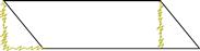
Figure 11.13 The imagined (yellow) additions to the parallelogram suggest a method for calculating the area of a parallelogram.

The addition of mental imagery to external imagery has a great many variations, and box [A3] gives only the most basic form of this algorithm. One of its limitations is our ability to mentally imagine additions to visualizations, and this is extremely restricted, at least for most people (Kosslyn, 1990). Because of this, much of the most flexible and creative visual thinking involves externalizing tentative solutions. This is called creative sketching, and we deal with it next.

Algorithm 4: Design Sketching

Sketching on paper, a blackboard, or a tablet computer is fundamental to the creative process of most artists, designers, and engineers. There is a huge difference between creative sketching and the production of a finished drawing. Creative sketches are thinking tools primarily composed of rapidly drawn lines that are mere suggestions of meaning (Kennedy, 1974; Massironi, 2004), whereas finished drawings are polished recordings of ideas that have already been fully developed.

Sketches can be considered as externalization of mental imagery. Someone who begins a sketch is literally trying to represent on paper something he has imagined. Because of the limitations of visual imaging (Kosslyn, 1990) what can be mentally imaged is quite simple. If something, however crude, that represents a mental image can be put down as a sketch, then additional elements can be mentally imaged as additions to what is already on the paper.

Sketches benefit from the abstract nature of lines. A line can represent an edge, a corner, or the boundary of a color region, as well as something quite abstract, such as the flow of people in a large store. Lines on the paper can be reinterpreted to have different meanings. A scribbled area on the sketch of a garden layout can be changed from lawn to patio to vegetable garden, simply by an act of imagination. The psychologist Manfredo Massironi (2004) invented an exercise that dramatically illustrates the ease with which the brain can interpret lines in different ways. First draw a scribble on a piece of paper—a single line with three or four large loops should be sufficient. Next, try to turn the scribble into a bird simply by adding a “<” and an “o.” In a surprising number of instances, the meaningless loops will become resolved into heads and wings and very satisfactory birds will result (see Figure 11.14).

[A4] Design sketching

Display environment: Paper and pencil or tablet computer.

Figure 11.14 The metamorphosis of scribbles. From Ware (2009), based on a concept by Massironi (2004). Reproduced with permission.

The creative sketching algorithm is set out in box [A4]. It involves a cycle in which concepts are externalized through marks on paper, then interpreted through analytic visual queries. Additions or deletions are mentally imaged so as to provide a low-cost way of testing new concepts in the context of those already set down. Those that pass the test will result in new externalizations. Sketches themselves are disposable; starting over is always an option.

Architects are known to be prolific sketchers, and Suwa and Tversky (1997) studied how they used sketches in the early stages of design. They found that a kind of analytic seeing was important and that there were often unintended consequences resulting from the placement of sketch lines. Sometimes these resulted in constructive solutions that had not been noticed previously.

An example of how sketching might be used in an architectural design project is given in Figure 11.15. The site constrains the basic footprint of the building to the two rectangles that have been roughly scribbled, as shown in Figure 11.15(a). The architect next imagines the main entrance in the center of the large rectangle, shown in Figure 11.15(b), but immediately realizes that the space needed for an entrance hall and its associated ticket offices will conflict with the client’s wish to have a great sculpture hall with windows looking out in that direction. The architect next imagines the entrance and entrance hall in the smaller rectangle and, because this works better, adds lines to externalize the concept.

Figure 11.15 (a) The entrance is imagined on the right. (b) An alternative is imagined with an entrance on left. (c) The solution is externalized.

For creativity to be supported, the medium used for design must afford tentative interactions. The lack of precision in quick, loose sketches actually allows for multiple interpretations. The sketches that people construct as part of the creative process are rapid, not refined, and readily discarded. Giving a child high-quality watercolor paper and paints is likely to inhibit creativity if the child is made aware of the expense and cautioned not to “waste” the materials. Schumann et al. (1996) carried out an empirical study of architectural perspective drawings executed in three different styles: a precise line drawing, a realistically shaded image, and a sketch. All of the drawings contained the same features and level of detail. The sketch version was rated substantially higher on measures of ability to stimulate creativity, changes in design, and discussions.

Algorithm 5: Brushing

It is often useful to represent data in several different views. Figure 11.16 is a complex display showing a graph of crime plotted against income level, a map view of crime statistics, a table view of more detailed numbers, and a histogram. Each of these views provides a different way of looking at the same set of numbers and each has advantages, but what if we want to relate patterns revealed in the scatterplot to locations on the map? This is a problem that can be solved by a method called brushing (Becker & Cleaveland, 1987). In brushing, selecting a data object in any one of the views causes those same data objects to be highlighted wherever they appear in all of the other views. The brushing algorithm is given in box [A5].

[A5] Brushing

Display environment: Data entities are represented in at least two different ways on different parts of the screen or on multiple screens.

1. Construct a visual query requiring information about a particular subset of the underlying data.

2. Select symbols representing the relevant subset of the data. As a result, the computer highlights all other representations of the data that has been selected.

3. Execute visual queries for task-relevant patterns in the highlighted representations. The queries may require information from two or more representations and be limited by visual working memory capacity.

Figure 11.16 The same data is displayed in four different ways, using a scatterplot, a histogram, a map, and a table. Selecting points in one view causes them to be highlighted in all other views. Courtesy of Dr. Mike de Smith (http://www.spatialanalysisonline.com/).

The goal of the brushing is to allow users to relate information patterns in one part of a compound display with patterns in another part. Information about those patterns must be stored in working memory (either visual or verbal) while attention is transferred. If the transfer of attention requires a visual search of even a few seconds, this can cause substantial loss of the working memory information and greatly reduce overall cognitive efficiency. For this reason, it is clearly essential that highlighting methods should support a rapid visual search.

A common problem is that composite displays of this kind are almost always visually complex; they are likely to already use a variety of line styles, colors, and textures, and this makes finding a visually distinctive highlighting method challenging. One solution is to use motion highlighting, assuming that motion is not already used in the data coding (Bartram & Ware, 2002). Motion has the advantage that it works well in the periphery of vision and it interferes little with the perception of color and shape.

Algorithm 6: Small Pattern Comparisons in a Large Information Space

A need to see detail in a larger context is a common problem for data visualization. The most common example is a map display, where we wish to compare small-scale features on the map. But, the same problem occurs with more abstract data, such as large network diagrams.

To solve this focus and context problem many systems afford epistemic actions that provide the user with a method for moving attention easily between detail and context views. In the previous chapter, we discussed zooming, adding extra linked windows, and other methods as a problem of mental geometry and found that some transformations are easier than others. In most cases, though, a much more important constraint on cognitive performance is imposed by visual working memory capacity.

To help analyze the problem of which focus and context interface is likely to be best we will take as a model the task of comparing patterns that are isolated small islands of information in a large geographical space. This is illustrated in Figure 11.17. The figure shows extra linked windows, placed so as to show two areas of detail.

Figure 11.17 Subwindows allow details to be compared while the overall context can also be seen (GeoZui3D interface).

A simpler alternative to having extra windows is a straightforward zooming interface. With a zooming interface, comparisons are made through rapid scale changes. The user must zoom in and look at one area of detail, hold the pattern (or part of it) in visual working memory, zoom out to get an overview and seek another pattern, and then zoom in again to make a comparison. The pattern in visual working memory is compared to new patterns found during the search process. If a possible match is found, it may be necessary to zoom in and out and back and forth to confirm details.

With the use of extra windows, as shown in Figure 11.17, parts of the main display are magnified. When two such windows are in position, it is possible simply to make eye movements between them to assess the relationship more rapidly.

The general algorithm for this task is given in box [A6]. It involves moving back and forth between patterns to make comparisons. This movement is an epistemic action that depends on the interface that has been provided. One way of implementing the epistemic action is through an interface that makes zooming rapid and easy. Another way is to provide support for extra magnifying windows. If two extra magnifying windows are used, they must be set up over pairs of patterns to make the comparison, but when the windows are in place the visual comparison can be made with much more rapid eye movements (Plumlee & Ware, 2002).

The critical resource here is visual working memory capacity, because this determines how many visits, back and forth, are required to make a comparison between a pair of patterns. If the master pattern is simple enough to be held in visual working memory, then zooming will often be more efficient, because it avoids the overhead of setting up multiple windows. If more than three visual-working-memory-sized chunks are in the master pattern, then it will be necessary to zoom back and forth between them, and the multiwindow solution will be faster.

[A6] Small pattern comparisons in a large information space

Display environment: A large data space with small isolated patterns that must be compared in some way.

In its simplest form, the time taken to perform this task is given by:

The number of comparison queries depends on the number of visual chunks in the patterns to be compared and on visual working memory capacity; for example, if there are seven visual chunks to be compared, the number of comparison queries will be three, because only three chunks can be stored in visual working memory to make a comparison. The first and second comparisons will involve three chunks each and the last will involve one chunk.

Plumlee and Ware (2002) modeled and predicted user performance on this task with the two interfaces we have been discussing—simple zooming vs. multiple windows. The number of zooms vs. window movements necessary to complete the task of finding identical clusters of simple shapes widely separated in a geographical space was estimated. Visual working memory was considered as a critical resource. The predictions of the model are shown in Figure 11.18 (left), modeled for capacities of visual working memory at two, three, and four items, leading to a range of predictions as shown by the broad colored wedges. When there are fewer visual chunks in the patterns to be compared, the zooming interface is best. As the number of chunks increases, the extra window interface is better. The crossover should be at about three chunks. The measured results, shown Figure 11.18 (right), closely matched the prediction.

Figure 11.18 Model predictions are shown on the left. Measured task performance is shown on the right. Multiple windows speed performance relative to the use of a zooming interface when the number of objects to be compared is five or more.

The model we have been describing here is greatly simplified. In fact, because eye movements have such a low cost, people act as if they are only comparing one object at a time (instead of three) with the multiple windows interface. They make many more eye movement than necessary and they also make far fewer errors (Plumlee & Ware, 2006). So the multiwindow solution is more reliable as well as faster.

Still, in many cases, detailed modeling is not necessary to decide if a user interface should support extra windows for detailed pattern comparisons. We can give the following rule of thumb:

[G11.3] In large data spaces containing small islands of critical information, consider enabling the user to add extra windows showing magnified areas of the larger space. This is especially useful for tasks that require frequent queries to compare patterns having more than three visual working memory chunks. This is a supplement to guideline G10.15.

Algorithm 7: Degree-of-Relevance Highlighting

Sometimes information objects in a display are interrelated in ways that are highly task relevant. If we inquire about a particular data object—say, a node representing a man who is a criminal suspect—then we also likely want to know about his known associates. Normally, the designer will group these related objects on the screen, but this is not always possible because of other design constraints, so related objects become distributed across the display. Also, there are many cases where the amount of information is such that a simplified representation of every data object can be placed on the screen but not with adequate clarity or detail.

In degree-of-relevance highlighting, we are interested in displaying all of the information on the screen at once, but because of its density it cannot all be made legible. A simple interaction solves the problem; touching an object causes both it and other task-relevant data objects to be highlighted, and the highlighted objects may also reveal additional detail. Degree of relevance is calculated using a computer algorithm designed to rate the task relevance of other entities in the database based on interaction history. The simplest version of this involves only the most recent selection.

One way that this approach has been employed is in network diagrams consisting of nodes and links. Most static diagrams contain fewer than 30 or so graphically represented entities and a similarly small number of lines linking or enclosing them. Having too many nodes and links makes it impossible to trace out the connections between them. Degree-of-relevance highlighting makes it possible to deal with much larger diagrams.

The Constellation system of Munzner et al. (1999) provides an example of how interactive degree-of-relevance highlighting can provide views into a very complex semantic network, far larger than can be displayed with static concept maps. Figure 11.19 shows a screen shot, but this static image does not do justice to the system. Constellation uses hover queries to allow for rapid highlighting of subsets of the graph. Links attached to a node become highlighted as the cursor passes over the node. In addition, when the user clicks on a particular node, closely related semantic concepts are allocated more screen space and larger fonts. In essence the computer provides a visual information scent, to use Pirolli and Card’s (1995) term, as a guide to the best place to search for more information. By using this technique, a large amount of semantic information can be accessed very quickly.

Figure 11.19 A screen image of the Constellation system (Munzner et al., 1999) showing a view into the MindNet semantic network database. (Reproduced with permission.)

Note that the rapid query techniques get around the usual problems of graph layout. Most of the work in graph layout is aimed at producing aesthetically pleasing drawings of graph structures by paying particular attention to minimizing edge crossings of nodes (Di Battista et al., 1998). A clear static graph drawing of the information in Figure 11.19 is probably impossible, because there are simply too many links. In Constellation, Munzer abandoned the usual criteria, allowing edges to cross each other and to cross nodes, using interactive techniques to reveal information as needed allowed visual access to much larger structures.

The MEgraph system is another example of degree-of-relevance highlighting (Ware & Bobrow, 2005; Ware et al., 2008). MEgraph used Fortune 500 companies as a test example, illustrated in Figure 11.20. This graph is actually a kind of social network, showing links between companies (colored dots) via members of the boards of directors (gray dots) for those companies. When board members are on the boards of more than one company, they form a high-level social link between the companies. In MEgraph, touching a node causes motion highlighting of the social links between nodes and the labels of the companies to appear. Users can choose to set the range of highlighting at one link, two links, or more. The reason why this approach makes sense is that in social networks we are mostly interested in short chain connections, making degree of relevance easy to compute—for example, who is a friend and who is a friend of a friend? Rarely is a chain longer than that; therefore, automatically highlighting these short chains will help users reason with the diagram.

[A7] Degree-of-relevance highlighting

Display environment: A display containing many symbols representing entities linked by a complex overlapping set of relationships.

1. Construct a visual query to find a symbol that may lead to useful information (information scent).

2. Execute an epistemic action by selecting a symbol.

3. Computer highlights all symbols with a high degree of relevance to selected symbol.

4. Execute a visual pattern query among highlighted symbols for additional information scent.

5. If a very high relevance symbol is found, execute an epistemic action to drill down for additional information. Usually this will be presented in a different display window.

6. Repeat from 1 as needed, cognitively marking visited symbols.

Figure 11.20 The MEgraph system uses motion as additional highlighting on the green lines and their attached nodes. This makes them independently searchable.

The degree-of-relevance highlighting algorithm is given in pseudocode in box [A7]. On average, the time taken to find a target on a single iteration of the main loop is given by

11.1

where p_h is the probability that the search target is in the highlighted set, and t_h is the time taken for the visual search. This can be very short if the target is a member of a small preattentively distinct set, but typically would not take more than a few seconds even if a serial search is needed. p_nh is the probability of finding the target when it is not highlighted, and t_nh is the time required to find that target. If a target is not highlighted, the search time may be much longer, perhaps by minutes, and so the value of the algorithm depends on how efficient the computer can be at finding task-relevant information.

Generally speaking, degree-of-relevance highlighting is useful to display data sets having between 30 and a few thousand entities. There is an upper limit on how much information can be represented on a screen. For example, it may take 100 pixels to draw a symbol, and for clarity a 5-pixel border may be required. This means that, given a 1-million pixel screen, we can represent at most 2500 symbols in a dense matrix, which is far too many to search efficiently. Searching that is not preattentive requires 40 msec per item, plus a 100-msec eye movement, for every 4 or 5 items, meaning that it will take minutes to conduct a visual search for a single symbol without some visual support. If a degree-of-relevance algorithm can reduce the visual search to around 10 to 20 items, then the gain in cognitive efficiency can easily be an order of magnitude.

Algorithm 8: Generalized Fisheye Views

A fisheye view is a display of an information space that has been geometrically distorted to show certain information larger and more clearly while shrinking other information. A generalized fisheye view is a much more powerful and abstract concept developed by George Furnas in one of the most influential papers published in the field of information display (Furnas, 1986). In a generalized fisheye view, the computer attempts to show only task-relevant information and hides or shrinks other information. The concept has nothing to do with geometry. Furnas called the function underlying what is shown a degree of interest (DOI) function. We will use the term degree of relevance instead, because it is useful to focus on task relevance when analyzing algorithms and because the interest of the user is much more difficult to determine.

A closely related concept is the adaptive level of detail display (Bishop & Tipping, 1998). In a level of detail display, information is assumed to be hierarchical so that an object can be expanded to expose ever greater amounts of detail. If a display system is adaptive, this means that the system automatically shows more detail for objects that are judged, according to some computational model, to be more task relevant. In general, an adaptive information visualization is any display that adapts based on some computer model of the user’s information needs.

[A8] Generalized fisheye views

Display environment: A set of symbols representing data entities drawn from a much larger set. The entities are linked by a complex overlapping set of relationships.

The algorithm for visual thinking with a generalized fisheye view is very similar to that for degree-of-relevance highlighting. The important difference is that in a generalized fisheye view less important information is completely hidden rather than being merely de-emphasized (as in box [A7]). The generalized fisheye view algorithm is given in box [A8]. On average, the time taken to find a target on a single iteration is given by

11.2

where p_d is the probability that the search target is displayed on the screen, and t_d is the time required for the visual search in that case. This can be very short if the target is a member of a small preattentively distinct set, but typically would not take more than a few seconds even if a serial search is needed because the algorithm has reduced the number of displayed objects to a small subset. Also, p_nd is the probability of finding the target when it is not on the screen, and t_nd is the time to find that target.

As with degree-of-relevance highlighting, the value of the generalized fisheye view algorithm depends entirely on the reliability with which the computer can predict the user’s information needs. Sometimes this is easy; for example, a user alert to a system problem may always be followed by a request from the system user for more detailed information about the originating component. If the system can automatically show that extra detail, work will become more efficient.

The downside of generalized fisheye views is that the algorithm will hide important information. Often the user’s goals cannot be easily inferred from their actions, and hiding the wrong information can have serious consequences. It may require a whole set of epistemic actions through menu selections, keyword searches, or other navigation methods to find what it needed. This can take an arbitrarily long time, so the success of adaptive level of detail methods obviously depends almost entirely on the success of the degree-of-relevance algorithm in keeping p_nd low.

One application of generalized fisheye views is in the adaptive display of large node–link diagrams (Schaffer et al., 1993; Bartram et al., 1994). In their intelligent zoom system (illustrated in Figure 11.21), a hierarchical network diagram is being examined. As parts of the network are expanded to see more detailed connections within components, other parts become more compact. If the user starts to explore other parts of the network, some of the boxes that had previously been opened will be closed to make room, hiding their contents.

Figure 11.21 A series of frames showing the intelligent zoom interface. Areas of interest expand when selected; other objects shrink accordingly. Redrawn from Schaffer et al. (1993).

Algorithm 9: Multidimensional Dynamic Queries with Scatter Plot

With multidimensional discrete data, all entities have the same set of attributes. The attributes define the data dimensions, and each entity can be thought of as a point in a multidimensional space. For example, a researcher interested in heart disease might have a data set from cardiac patients including measurements of blood chemistry, as well as statistics on blood pressure, alcohol intake, and other variables for every patient. Each measurement defines a data dimension, and each patient becomes a point in a multidimensional space defined by the dimensions. Techniques discussed previously such as enhanced scatterplots or parallel coordinates can be used to display the data, but if the data set is large it will be impossible to visualize in its entirety.

Ahlberg et al. (1992) developed an interface that enables a researcher to narrow down the set of points that is displayed using a set of sliders, one for each data dimension. Each slider adjustment is an epistemic action, narrowing the range of what is displayed. They called the interactive hiding and revealing of data in this way dynamic queries, and they demonstrated it with a number of interactive multivariate scatterplot prototypes. It also became the basis for the Spotfire^® product. Figure 11.22 shows an example of it in the form of the FilmFinder demonstration application. This provides the user with a slider to select on the basis of movie length, another to select on the basis of year of production, and more to select actor and director names.

Figure 11.22 The FilmFinder application of Ahlberg and Shneiderman (1994) used dynamic queries to allow rapid interactive updating of the set of data points mapped from the database to the scatterplot display in the main window. Courtesy of Matthew Ward.

The basic algorithm for multidimensional dynamic queries with a scatterplot is given in box [A9]. It involves epistemic actions using interactive slider bars to narrow down the displayed subset of the data space in order to find a small set of symbols that represent the most relevant data. The goal is to reduce the number of displayed points to a manageable size. At this point, a visual pattern search can be made for critical patterns. Ultimately, each of a small set of points may be individually selected to get complete detailed information by means of additional epistemic actions.

We can roughly estimate the size of the database for which this method is useful. The sliders tend to be quite short, because of limitations in available screen space, and this limits the amount of selection that can be imposed. Perhaps, as a rule of thumb, each slider enables us to restrict the search to 10% of the targets on a particular dimension. This means that the overall restriction on what is displayed is 0.1^d, where d is the number of data dimensions. If there are four dimensions, the reduction in the number of targets will be a factor of 10,000.

There are also limitations on the number of sliders that can be meaningfully used before the fluidity of the process becomes compromised. Let’s put this limit, arbitrarily, at 10. In addition, let’s assume that we would like fewer than 10 targets remaining on the screen at the end of the interactive process as candidates for detailed examination. In this extreme example, a data set containing 100 billion items might be dealt with interactively.

As a final observation, there is no reason why interactive range selection has to be coupled only with scatterplots. The same visual thinking algorithm applies to parallel coordinates, where the sliders are placed directly on the parallel axes (Inselberg & Dimsdale, 1990). Also, interactive range selection using a slider can be applied to any other visualization where it is desirable to restrict what is shown according to some continuously varying attribute.

[A9] Multidimensional dynamic queries with scatterplot

Display environment: A scatterplot with symbols representing entities drawn from a set of multidimensional discrete data, with a set of controls that restricts the range displayed on each of the data dimensions.

Algorithm 10: Visual Monitoring Strategies

Supervisory control is a term used to describe a situation where a semiautonomous system, such as a plane on autopilot or a chemical plant, runs with only occasional input from a human operator. In supervisory control systems, operators must monitor a set of instruments every so often. The basic visual thinking algorithm involves a user setting up a schedule of self-interrupts, according to which they will periodically stop whatever else they are doing and conduct a visual scan of a set of displays looking for anomalous patterns that may require action. Once such a pattern is found the appropriate action is taken.

Models developed to account for operators’ visual scanning strategies generally have the following elements (Wickens, 1992):

Channels. These are the different ways in which the operator can receive information. Channels can be display windows, dials on an instrument panel, or nonvisual outputs, such as loudspeakers (used for auditory warnings). (Note that this meaning is different from the concept of perceptual channels discussed in this book.)

Events. These are the signals occurring on channels that provide useful information.

Expected cost. This is the cost of missing an event. System operators base their monitoring of different channels on a mental model of system event probabilities and the expected costs of these (Moray & Rotenberg, 1989; Wickens, 1992). Charbonnell et al. (1968) and Sheridan (1972) proposed that monitoring behavior is controlled by two factors: the growth of uncertainty in the state of a channel (between samples) and the cost of sampling a channel. Sampling a channel involves fixating part of a display and extracting the useful information. The cost of sampling is inversely proportional to the ease with which the display can be interpreted. This model has been successfully applied by Charbonnell et al. (1968) to the fixation patterns of pilots making an instrument landing.

Two other factors may influence visual scanning patterns:

Operators may minimize eye movements. The cost of sampling is reduced if the points to be sampled are spatially close. Russo and Rosen (1975) found that subjects tended to make comparisons most often between spatially adjacent data. If two indicators are within the same effective field of view, this tendency will be especially advantageous.

There can be oversampling of channels on which infrequent information appears (Moray, 1981). This can be accounted for by short-term memory limitations. Because it requires significant cognitive effort to keep a particular task in mind, people can reliably monitor an information channel on a frequent self-interrupt schedule (e.g., every minute), but they are much less reliable when asked to monitor an event every 20 minutes, presumably because the self-interrupt program is lost from working memory. To compensate, operators may sample more frequently than required.

One solution that can assist system operators in being more reliable is for a computer system to provide visual or auditory reminders at appropriate intervals as an alternative to internal mental interrupts. In addition, if a system can determine when additional attention from an operator is needed this can be signaled. One good way of doing this is to use motion cues, since motion in the periphery of vision is readily detected and different levels of urgency can be expressed (Ware et al., 1992).

The limits of attention and visual working memory capacity mean that well-designed monitoring procedures can break down under extreme conditions. Operators may exhibit dysfunctional behaviors in high-stress situations. Moray and Rotenberg (1989) suggested that under crisis conditions operators cease monitoring some channels altogether. In an examination of control room emergency behavior, they found that under certain circumstances an operator’s fixation would become locked on a feedback indicator, waiting for a system response at the expense of taking other more pressing actions.

Conclusion

The ten visual thinking algorithms set out in this chapter are greatly simplified sketches developed to encourage thinking about cognitive tool design in a more process-orientated way. They do not spell out every mouse click or working memory operation. Other methods have been developed that are much more complete and detailed. In particular, the ACT-R model (Anderson et al., 1997) can be used to create a more complete account of the visual and cognitive operations involved in performing particular tasks. But, the cost of using a system like ACT-R is the effort involved in setting up a very detailed cognitive model of task execution. This can take days or weeks, and the process is incompatible with rapid prototype development, a method that usually produces the best designs. The alternative offered here in the form of visual thinking algorithms is intended to provide a framework for rough and ready calculations that can be done in minutes on scraps of paper. This can be done as part of prototype development in order to understand the critical bottlenecks restricting cognitive productivity.

Once we begin to think in terms of visual thinking algorithms it becomes clear that a common bottleneck in cognitive processing comes from the limitations of working memory capacity. This is the reason why it is so essential to enable people to rapidly move attention from one meaningful pattern to another. If we could hold more in our heads, we would not need to shift attention so often. Providing interactive methods that work around the limits of working memory capacity can, in many cases, result in impressive gains in efficiency. For example, adding extra windows for comparing patterns side by side using rapid eye movements instead of slow zooming can provide very substantial gains (Algorithm 6). Degree-of-relevance highlighting means that a network diagram ten times as large can be handled on a single screen (Algorithm 7). Without it, some other method would have to be used, such as zooming, and this would greatly increase both the time and the working memory load.

As a final comment, the person who wishes to design an interactive visualization must contend with two sets of conflicting forces. On the one hand, there is the requirement for the best possible visual solution, tailored exactly to the problem to be solved. On the other hand, there is the need for consistency in representation and interaction style. This need is even greater when large, international organizations have a common set of goals that demand industrywide visualization standards. At the stage of new discoveries in information visualizations, standardization is the enemy of innovation and innovation is the enemy of standardization. It is important that we get the research done before the standards are formed; otherwise, it will be too late. These are exciting times for information visualization, because we are still in the discovery phase, although this phase will not last for long. In the next few years, the wild inventions that are now being implemented will become standardized. Like clay sculptures that have been baked and hardened, the novel data visualization systems of today’s laboratory will become cultural artifacts, everyday tools of the information professional.