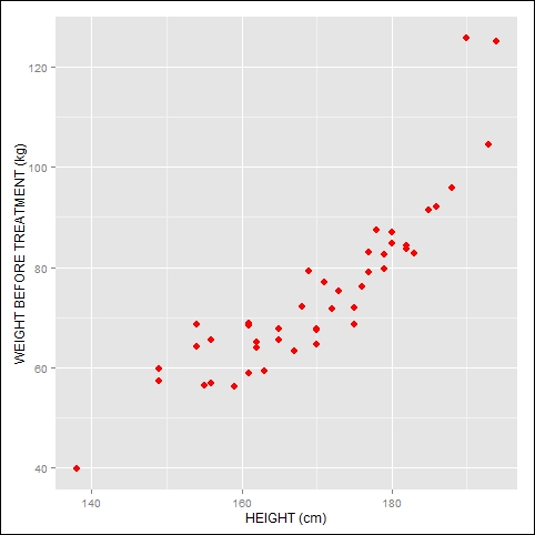
Let's start with a simple example where we use the medical dataset that we saw in Chapter 2, Advanced Functions in Base Graphics. Again we cut and paste from the code file for this chapter. We invoke the ggplot2 library, set up a simple scatterplot using red symbols, and save it as a PNG file. The syntax for invoking the library is as follows:
library(ggplot2)
Now let's plot HEIGHT against WEIGHT_1, using I() for color and symbol size. We choose red and a symbol size three times the qplot default size. Enter this syntax on the R command line:
qplot(HEIGHT, WEIGHT_1, data = T, xlab = "HEIGHT (cm)", ylab = "WEIGHT BEFORE TREATMENT (kg)" , color = I("red"), size = I(3))
After running the preceding command, you will get the following graph:

We get a scatterplot by default (that is, without specifying any geom argument). We see a plotting background that is gray in color and includes a grid. This is the default plotting background for qplot. Now let's save the graph as a PNG file with filename fig_1.png. You probably want to save your graph in a particular directory. To do so, you must ensure that this directory becomes your R "working directory".
You can set your R working directory by navigating to File | Change Dir and selecting the directory you wish to use. Now, enter these commands on the R command line:
png(filename = "fig_1.png")
qplot(HEIGHT, WEIGHT_1, data = T, xlab = "HEIGHT (cm)", ylab = "WEIGHT BEFORE TREATMENT (kg)" , color = I("red"), size = I(3))
dev.off()
Check your working directory to see whether the graph has been saved there.