Chapter 14
Performance Optimization of an Image Analysis Application
Introduction
Chapter 13 discussed step by step how to use AMD CodeAnalyst, Profiler, gDEBugger, and KernelAnalyzer to profile and debug an OpenCL application. While Chapter 13 gave a very basic introduction to the tools, in this chapter, we use a real-world application as an example to walk through the steps from migrating a single-threaded application to one that utilizes the GPU and APU power using OpenCL. We will see how some of the profiling techniques that these, and other, tools provide can be used to investigate bottlenecks and improve peak performance of an application. After all, high performance is generally the reason to put time into porting code to use OpenCL.
This chapter dives into detailed profiling techniques provided by the software development tools described in Chapter 13, and applies them to a real application. We port a medical image analysis pipeline from a traditional CPU multithreaded execution and optimized for execution in OpenCL on a GPU. In this chapter, we see both static analysis and profiling and the trade-offs involved in optimizing a real application for data-parallel execution on a GPU.
In this chapter, we use AMD tools as an example. More thorough descriptions of all the tools are available in their documentation, and tools from other vendors provide similar capabilities. You should use whatever tools are appropriate for the architecture you are targeting.
We present a vasculature image enhancement module, which is the first and most important step for a vessel analysis application. The automatic and real-time enhancement of the vessels potentially facilitates diagnosis and later treatment of vascular diseases. The performance and power consumption of the proposed algorithms are evaluated on single-core CPU, multicore CPU, discrete GPU, and finally an accelerated processing unit (APU).
In this chapter, we first discuss the algorithm to give a background to the problem being solved. We then show how the CPU implementation may be ported to OpenCL and run on a GPU. In this section, we show how different tools may be used to inform the developer about what parts of the application should move to OpenCL and how to optimize them once they are there. We examine some trade-offs in kernel code and how they affect performance. Finally, we see how these changes may affect energy use by the application and show that the GPU can give an energy consumption benefit.
Description of the algorithm
The algorithm chosen is a coarse segmentation of the coronary arteries in CT images based on a multiscale Hessian-based vessel enhancement filter (Frangi, 2001). The filter utilizes the second-order derivatives of the image intensity after smoothing (using a Gaussian kernel) at multiple scales to identify bright tubular-like structures. The six second-order derivatives of the Hessian matrix at each voxel can be either computed by convolving the image with second-order Gaussian derivatives at preselected scale value or approximated using a finite difference approach.
Various vessel enhancement techniques have been proposed in the past decade. Three of the most popular techniques for curvilinear structure filtering have been proposed by Frangi (2001), Lorenz et al (1997), and Sato et al (1998). All these approaches are based on extracting information from the second-order intensity derivatives at multiple scales to identify local structures in the images. Based on that information, it is possible to classify the local intensity structure as tubular-like, plane-like, or block-like.
In this chapter, we use a multiscale Hessian-based vessel enhancement filter by Frangi (2001) because of its superior performance compared with other tubular filters (Olabarriaga et al. 2003). The filter utilizes the second-order derivatives of the image intensity after smoothing using a Gaussian kernel at multiple scales to identify bright tubular-like structures with various diameters. The six second-order derivatives of the Hessian matrix at each voxel are computed by convolving the image with the second-order Gaussian derivatives at preselected scales.
Assuming a continuous image function I(x), x = (x,y,z), the Hessian matrix H for the 3D image at any voxel x is defined as

At a predefined scale σ, Hessian H can be computed by convolving the image I(x) with the second-order Gaussian derivatives shown in Figure 14.1(a).
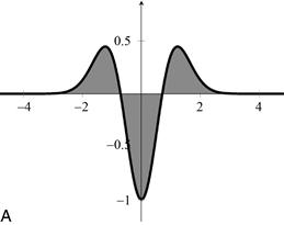

Figure 14.1 Illustrations of second-order Gaussian derivative and ellipsoid. (a) The second-order derivative of a Gaussian kernel at scale σ = 1. (b) The ellipsoid that locally describes the second-order structure of the image with illustration of the principal directions of curvature.
A vesselness term vσ(x) is defined as in Frangi (2001) and is based on the eigenvalues and eigenvectors of Hσ(x). Let |λ1| ≤ |λ2| ≤ |λ3| denote the eigenvalues of the Hessian Hσ(x), and v1, v2, v3 are the corresponding eigenvectors. The principal curvature directions are then given by v2 and v3, as shown in Figure 14.1(b).
Since arteries have higher intensity values in computerized tomographic angiography (CTA) images than surrounding soft tissues, the vessel center points are the ones with maximal local intensities after smoothing. Thus, the corresponding eigenvalues λ2 and λ3 should be negative for voxels on the arteries in CTA image; otherwise, the vesselness response should be zero. As in Frangi (2001), the vesselness response vσ(x) at voxel x with scale σ is formulated as

where 
Controlled by α, parameter A discriminates plate-like from line-like structures; B, dominated by β, accounts for deviation from blob-like structures, and S, controlled by γ, differentiates between high-contrast region, for example, one with bright vessel structures on a dark background, and low-contrast background regions. This approach achieves scale normalization by multiplying H by σ2 before eigenvalue decomposition. The weighting factors α, β, and γ are to be specified in order to determine the influence of A, B, and S.
Because the size of the cross-sectional profile of the coronaries varies substantially from the root to the distal end, a single-scale vesselness response is not sufficient to capture the whole range of coronaries. The vesselness response of the filter reaches a maximum at a scale that approximately matches the size of the vessel to detect. Thus, integrating the vesselness response at different scales is necessary to support varying vessel sizes. Here, the response is computed at a range of scales, exponentially distributed between σmin and σmax. The maximum vesselness response Vσ(x) with the corresponding optimal scale σoptimal(x) is then obtained for each voxel of the image:

The scale σoptimal (x) approximates the radius of the local vessel segment centered at x. There are two groups of outputs of this vessel enhancement algorithm:
(1) The final vesselness image denoted as Iv is constructed using the maximum response Vσ(x) of each voxel x as the intensity value;
(2) The optimal scale σoptimal(x) is selected for each voxel x (Figure 14.2).

Figure 14.2 Flowchart of the vessel enhancement algorithm described in this chapter.
In this chapter, we use a 3D cardiac CTA image with voxel dimensions 256 by 256 by 200, voxel resolution 0.6 × 0.6 × 0.5 mm3.
Migrating multithreaded CPU implementation to OpenCL
At the time of writing, AMD offers the following development tools: APP KernelAnalyzer, CodeAnalyst, APP Profiler, and gDEBugger. The first two are used in this section to port the multithreaded CPU-based image analysis application to GPU. The APP Profiler will be utilized in the next section for performance optimization.
KernelAnalyzer is a static analysis tool for viewing details about OpenCL kernel code (among other possible inputs). It compiles the code to both AMD’s intermediate language and the particular hardware ISA of the target device and performs analyses on that data such that it can display various statistics about the kernel in a table. This can be useful for catching obvious issues with the compiled code before execution as well as for debugging compilation.
CodeAnalyst is traditionally a CPU profiling tool that supports timer-based and counter-based sampling of applications to build up an impression of the application’s behavior. Recent editions of CodeAnalyst have added support for profiling the OpenCL API.
The APP Profiler supports counter-based profiling for the GPU. The approach it uses is not interrupt based in the way that CodeAnalyst is, rather it gives accumulated values during the execution of the kernel. This information is useful for working out where runtime bottlenecks are, in particular, those arising from computed memory addresses that are difficult or impossible to predict offline.
Finally, gDEBugger is a debugging tool that supports step-through debugging of OpenCL kernels.
Hotspot Analysis
Before implementing and optimizing for GPU and APU platforms, we first need to identify the hot spots in the multithreaded CPU-based implementation with the time-based profiling (TBP) facility in CodeAnalyst. These hot spots are the most time-consuming parts of a program that are the best candidates for optimization.
At the time of writing, CodeAnalyst 3.7 offers eight predefined profile configurations, including time-based profile, event-based profile (access performance, investigate L2 cache access, data access, instruction access, and branching), instruction-based sampling and thread profile. It also offers three other profile configurations that can be customized. The profile configuration controls which type of performance data to be collected. For example, if we are interested in finding detailed information about the mispredicted branches and subroutine returns, the “investigate branching” configuration is the ideal choice. Note that you can also profile a Java or OpenCL application in CodeAnalyst to help identify the bottlenecks of your applications.
Here we focus on getting an overall assessment of the performance of this application and identifying the hot spots for further investigation and optimization purpose. Hence, two configurations suit our requirement: access performance and time-based profiling.
In TBP, the application to be analyzed is run at full speed on the same machine that is running CodeAnalyst. Samples are collected at predetermined intervals to be used to identify possible bottlenecks, execution penalties, or optimization opportunities.
TBP uses statistical sampling to collect and build a program profile. CodeAnalyst configures a timer that periodically interrupts the program executing on a processor core using the standard operating system interrupt mechanisms. When a timer interrupt occurs, a sample is created and stored for postprocessing. Postprocessing builds up an event histogram, showing a summary of what the system and its software components were doing. The most time-consuming parts of a program will have the most samples, as there would be more timer interrupts generated and more samples taken in that region. It is also important to collect enough samples to draw a statistically meaningful conclusion of the program behavior and to reduce the chance of features being missed entirely.
The number of TBP samples collected during an experimental run depends upon the sampling frequency (or, inversely, on the timer interval) and the measurement period. The default timer interval is one millisecond. Using a one millisecond interval, a TBP sample is taken on a processor core approximately every millisecond of wall clock time. The timer interval can be changed by editing the current time-based profile configuration. By specifying a shorter interval time, CodeAnalyst can take samples more frequently within a fixed-length measurement window. However, the overhead of sampling will increase too, which leads to higher load on the test system. The process of taking samples and the incurred overhead have an intrusive effect that might perturb the test workload and bias the statistical results.
The measurement period refers to the length of time over which samples are taken. It depends upon the overall execution time of the workload and how CodeAnalyst data collection is configured. The measurement period can be configured to collect samples for all or part of the time that the workload executes. If the execution time of a program is very short (for example, less than 15 s), it helps to increase program runtime by using a larger data set or more loop iterations to obtain a statistically useful result. However, it depends on the characteristics of the workload being researched to decide how many samples should be taken at what interval that would provide sufficient information for the analysis and, in some circumstances, increasing the length of the workload’s execution may change the behavior enough to confuse the results.
The system configuration for this work is an AMD Phenom II X6 1090T, Radeon HD 6970, with CodeAnalyst Performance Analyzer for Windows version 3.5.
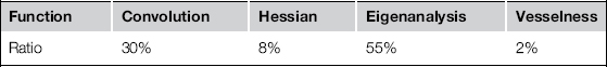
The access performance configuration shows 95% average system CPU utilization and 44% average system memory utilization. Given that TBP provides a system-wide profiling, to use the information provided in TBP efficiently, we need to select the entries corresponding to the application itself and perform postanalysis. The table below provides the four most time-consuming segments of the application, accounting for 95% of the application runtime. It also illustrates the percentage of function execution over the execution time of the whole application. Given that all these routines are inherently parallel for an image analysis workload, we can start by porting the eigenanalysis function into an OpenCL kernel first, followed by the convolution, Hessian, and vesselness computations.
Kernel Development and Static Analysis
In this chapter, we use the latest release of AMD APP KernelAnalyzer, version 1.12. KernelAnalyzer is a tool for analyzing the performance of OpenCL kernels for AMD Radeon Graphics cards. It compiles, analyzes, and disassembles the OpenCL kernel for multiple GPU targets and estimates the kernel performance without having to run the application on actual hardware or, indeed, having the target hardware in your machine. You can interactively tune the OpenCL kernel using its GUI. It is very helpful for prototyping OpenCL kernels in KernelAnalyzer and seeing in advance what compilation errors and warnings would be generated by the OpenCL runtime and subsequently for inspecting the statistics derived by analyzing the generated ISA code.
A full list of the compiler statistics can be found in the documentation of the KernelAnalyzer on AMD’s Web site. Here we illustrate a subset of them that are important for providing hints for optimizing this application:
1. GPR shows the number of general purpose registers used or allocated. The impact of GPR usage on the kernel performance is discussed later in this chapter.
2. CF shows the number of control flow instructions in the kernel.
3. ALU:Fetch ratio shows whether there is likely to be extra ALU compute capacity available to spare. ALU:Fetch ratios of 1.2 or greater are highlighted in green and those of 0.9 or less are highlighted in red.
4. Bottleneck shows whether the likely bottleneck is ALU operations or global memory fetch operations.
5. Throughput is the estimated average peak throughput with no image filtering being performed.
Figure 14.3 shows the KernelAnalyzer user interface while analyzing the vesselness OpenCL kernel.

Figure 14.3 KernelAnalyzer user interface while analyzing the vesselness kernel and generating output for the Radeon HD6970 (Cayman) GPU.
After developing all four major functions from this application in OpenCL and having it run on the GPU device, we inspect the performance of this newly migrated application in APP Profiler. Figure 14.4 shows the timeline view from APP Profiler. From the collected trace file, we can derive that the kernel execution takes 35.1% of the total runtime, the data transfer 32.7%, launch latency 9%, and other unaccounted activities that cover the setup time, and finalization time on the host-side account for the rest. We can see from the second to the last row of the trace that considerable time is spent copying data to and from the device. Given that all four functions are executed on device side and no host-side computation is left in between the kernels, we can safely eliminate the all interim data copies. This optimization reduces the total runtime by 23.4%. The next step is to inspect individual kernels and optimize them.

Figure 14.4 Execution trace of the application showing host code, data transfer, and kernel execution time using the timeline view of AMD APP Profiler.
Performance optimization
APP Profiler has two main functionalities: collecting application trace and GPU performance counters. Counter selections include three categories: General (wavefronts, ALUInsts, FetchInsts, WriteInsts, ALUBusy, ALUFetchRatio, ALUPacking), GlobalMemory (Fetchsize, CacheHit, fetchUnitBusy, fetchUnitStalled, WriteUnitStalled, FastPath, CompletePath, pathUtilisation), and LocalMemory (LDSFetchInsts, LDSWriteInsts, LDSBankConflict). For more detailed information about each of these counters, we refer to the APP Profiler documentation. In the rest of this section, we first discuss how to use kernel occupancy (a very important estimation provided in application trace) and a subset of GPU performance counters to guide the optimization.
Kernel Occupancy
This section provides an overview of the kernel occupancy calculation, including its definition and a discussion on the factors influencing its value and interpretation.
Kernel occupancy is a measure of the utilization of the resources of a compute unit on a GPU, the utilization being measured by the number of in-flight wavefronts, or threads as the hardware sees them, for a given kernel, relative to the number of wavefronts that could be launched, given the ideal kernel dispatch configuration depending on the workgroup size and resource utilization of the kernel.
The kernel occupancy value estimates the number of in-flight (active) wavefronts NwA on a compute unit as a percentage of the theoretical maximum number of wavefronts NwT that the compute unit can execute concurrently. Hence, the basic definition of the occupancy (O) is given by

The number of wavefronts that are scheduled when a kernel is dispatched is constrained by three significant factors: the number of GPRs required by each work item, the amount of shared memory (LDS for local data store) used by each workgroup, and the specified workgroup size.
Ideally, the number of wavefronts that can be scheduled corresponds to the maximum number of wavefronts supported by the compute unit because this offers the best chance of covering memory latency using thread switching. However, because the resources on a given compute unit are fixed and GPRs and LDS are hence shared among workgroups, resource limitations may lead to lower utilization. A workgroup consists of a collection of work items that make use of a common block of LDS that is shared among the members of the workgroup. Each workgroup consists of one or more wavefronts. Thus, the total number of wavefronts that can be launched on a compute unit is also constrained by the number of workgroups, as this must correspond to an integral number of workgroups, even if the compute unit has capacity for additional wavefronts. In the ideal situation, the number of wavefronts of a particular kernel that the compute unit is capable of hosting is an integral multiple of the number of wavefronts per workgroup in that kernel, which means that the maximum number of wavefronts can be achieved. However, in many situations this is not the case. In such a case, changing the number of work items in the workgroup changes the number of wavefronts in the workgroup and can lead to better utilization.
The factors that dominate kernel occupancy vary depending on the hardware features. In the following discussion, we focus on two major AMD GPU architectures: VLIW5/VLIW4 and Graphics Core Next.
Kernel Occupancy for AMD Radeon HD5000/6000 Series
The Radeon HD5000 and Radeon HD6000 series are based on a VLIW architecture such that operations are scheduled statically by the compiler across 4 or 5 SIMD ALUs. In this section, we discuss how this architecture affects some of the statistics.
In the case that the LDS is the only constraint on the number of in-flight wavefronts, the compute unit can support the launch of a number of in-flight workgroups given by
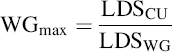
where WGmax is the maximum number of workgroups on a compute unit, LDSCU is the shared memory available on the compute unit, and LDSWG is the shared memory required by the workgroup based on the resources required by the kernel. The corresponding number of wavefronts is given as

where WFmax is the maximum number of wavefronts, WGmax is the maximum number of workgroups, and WFWG is the number of wavefronts in a workgroup.
There is also another constraint whereby a compute unit can only support a fixed number of workgroups, a hard limit of WGmax = 8. This also limits the effectiveness of reducing the workgroup size excessively, as the number of wavefronts is also limited by the maximum workgroup size. Currently, the maximum workgroup size is 256 work items, which means that the maximum number of wavefronts is 4 when the wavefront size is 64 (and 8 when the wavefront size is 32).
Thus, when the only limit to the number of wavefronts on a compute unit is set by the LDS usage (for a given kernel), then the maximum number of wavefronts (LDS limited) is given by

Another limit on the number of active wavefronts is the number of GPRs. Each compute unit has 16384 registers or 256 vector registers. These are divided among the work items in a wavefront. Thus, the number of registers per work item limits the number of wavefronts that can be launched. This can be expressed as
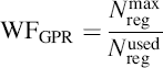
where Nreg is the number of registers per work item; the superscripts “max” and “used” refer to the maximum number of registers and the actual number of registers used per wavefront.
As the number of in-flight wavefronts is constrained by the workgroup granularity, the number of GPR-limited wavefronts is given by

Another limit on the number of in-flight wavefronts is the flow control stack. However, this is generally an insignificant constraint, only becoming an issue in the presence of very deeply nested control flow, and so we do not consider it here.
The final factor in the occupancy is the workgroup size, as briefly discussed above. If there are no other constraints on the number of wavefronts on the compute unit, the maximum number of wavefronts is given by

where WFmaxCU is the maximum number of wavefronts on the compute unit and WFWGmax is the maximum number of wavefronts on a compute unit when workgroup size is the only constraint.
This equation shows that having a workgroup size where the number of wavefronts divides the maximum number of wavefronts on the compute unit evenly generally yields the greatest number of active wavefronts, while indicating that making the workgroup size too small yields a reduced number of wavefronts. For example, setting a workgroup consisting of only 1 wavefront yields only 8 in-flight wavefronts, whereas (for example, given a maximum number of wavefronts on the compute unit of 32) a workgroup of 2 wavefronts will yield 16 wavefronts. Furthermore, having a single wavefront per workgroup doubles the LDS usage relative to having 2 wavefronts per workgroup as the LDS is shared only among the wavefronts in the same workgroup. Reuse of LDS may be a good thing for performance, too, reducing the number of times data is loaded from memory.
Given these constraints, the maximum number of in-flight wavefronts is given by

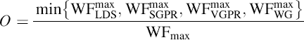
Thus, the occupancy, O, is given by:

The occupancy shown here is the estimated occupancy on a single compute unit. It is independent of the workloads on the other compute units on the GPU, as the occupancy is only really meaningful if there are sufficient work items to require all the resources of at least one compute unit. However, ideally, there should be a sufficient workload to ensure that more than one compute unit is needed to execute the work to explore the benefits of parallel execution. Higher occupancy allows for increased global memory latency hiding, as it allows wavefronts being swapped when there are global memory accesses. However, once there is a sufficient number of wavefronts on the compute unit to hide any global memory accesses, increasing occupancy may not increase performance.
Kernel Occupancy for AMD Radeon™ HD 7000
The Radeon HD7000 series is based on the Graphics Core Next architecture discussed in Chapter 6. This design separates the four VLIW-dispatched vector ALUs from the VLIW4-based designs and breaks it down into four separate SIMD units that are runtime scheduled. In addition, there is a separate scalar unit to manage control flow.
As a result of these architectural differences, the computation of occupancy on the HD7000 series GPUs differs in a number of significant ways from the previous occupancy calculation. While some features, such as the GPR, are still computed on the basis of individual SIMDs, these must be scaled to the whole compute unit. On the other hand, workgroup limits must be computed over the whole compute unit.
The first limit to the number of active wavefronts on the compute unit is the workgroup size. Each compute unit has up to 40 slots for wavefronts. If each workgroup is exactly one wavefront, then the maximum number of wavefronts WFmax is 40.
Otherwise, if there is more than one wavefront (WF) per workgroup (WG), there is an upper limit of 16 workgroups (WG) per compute unit (CU). Then, the maximum number of wavefronts on the compute unit is given by

where WFWG is the number of wavefronts per workgroup.
The second limit on the number of active wavefronts is the number of VGPR (vector GPR) per SIMD.

where VGPRmax is maximum number of registers per work item and VGPRused is the actual number of registers used per work item. However, for the total number of wavefronts per compute unit, we have to scale this value by the number of compute units:

At the same time, the number of wavefronts cannot exceed WFmax, so

However, the wavefronts are constrained by workgroup granularity, so the maximum number of wavefronts limited by the VGPR is given by

The third limit on the number of active wavefronts is the number of SGPR (Scalar GPR). SGPRs are allocated per wavefront but represent scalars rather than wavefront-wide vector registers. It is these registers that the scalar units discussed in Chapter 6 use. The SGPR limit is calculated by

The final limit on the number of active wavefronts is the LDS. The LDS limited number of wavefronts is given by

where WGmax is the maximum number of workgroups determined by the LDS. Then, the maximum number of wavefronts is given by

Thus, the occupancy, O, is given by
Impact of Workgroup Size
The three graphs in Figure 14.5 provide a visual indication of how kernel resources affect the theoretical number of in-flight wavefronts on a compute unit. This figure is generated for the convolution kernel with workgroup size of 256 and 20 wavefronts on a Cayman GPU. The figure is generated directly by the profiler tool and its exact format depends on the device. There will be four subfigures if the kernel is dispatched to an AMD Radeon™ HD 7000 series GPU device (based on Graphics Core Next Architecture/Southern Islands) or newer. In this case, the extra subfigure is “Number of waves limited by SGPRs” that shows the impact of the number of scalar GPRs used by the dispatched kernel on the active wavefronts.

Figure 14.5 A visualization of the number of wavefronts on a compute unit as limited by (a) workgroup size, (b) vector GPRs, (c) LDS. This figure is generated by the AMD APP Profiler tool. The highlight on the title of (a) shows that the workgroup size is the limiting factor in this profile.
The title of the subfigure representing the limiting resource is highlighted. In this case, the highlight is placed on the first subfigure: “Number of waves limited by workgroup size.” More than one subfigure’s title is highlighted if there is more than one limiting resource. In each subfigure, the actual usage of the particular resource is highlighted with a small square.
The first subfigure, titled “Number of waves limited by workgroup size,” shows how the number of active wavefronts is affected by the size of the workgroup for the dispatched kernel. Here the highest number of wavefronts is achieved when the workgroup size is in the range of 128–192. Similarly, the second and third subfigures show how the number of active wavefronts is influenced by the number of vector GPRs and LDS used by the dispatched kernel. In both case, as the amount of used resource increases, the number of active wavefronts decreases in steps.
In the same APP Profiler occupancy view, just below Figure 14.5, a table as shown below is generated with device, kernel information, and kernel occupancy. In the section “Kernel Occupancy,” the limits imposed by each resource are shown, as well as which resource is currently limiting the number of waves for the kernel dispatch, with the occupancy ratio estimated in the last row.

Given this analysis provided by the kernel occupancy view, the limiting factors would be the optimization target. To keep it simple and for illustration purpose, we lower the workgroup size to 128 instead of 192 to check whether we can eliminate workgroup size as the limiting factor. A large workgroup size may not, after all, be necessary if enough wavefronts are present to cover memory latency. After this modification, we obtain a new set of kernel occupancy information as shown Figure 14.6, where the small square marks the current configuration with workgroup size 128 and wavefronts 16.


Figure 14.6 The same visualization as in Figure 14.5 but where the workgroup size is lowered to 128. All three factors now limit the occupancy.
This change has a negative impact on the occupancy ratio, and all three factors are now limiting the number of active wavefronts. However, using APP Profiler, we can collect not only application trace but also the GPU performance counters. Table 14.1 shows a subset of the details that can be obtained from collecting GPU performance counters. Note that this table is based on the first configuration with workgroup size {64, 4, 1}, or a flattened workgroup size of 256 work items. Here four kernels are executed five times, each giving the gradual increase of the sigma value as described in the algorithm section. This trace does not include interim data transfers between kernels. As we discussed earlier, those interim transfers can be eliminated once all computations are performed on GPU device and so here we see only the first transfer from host to device and the end result being copied back after the data is processed.
Table 14.1 A subset of the hardware performance counter values obtained from a profiling run.

In Table 14.1, we see more information than we have yet discussed. In summary,
Global work size and workgroup size are the NDRange parameters used for the kernel dispatch.
ALUBusy is the percentage of the execution during which the vector ALUs are being kept busy with work to do. If all the wavefronts on the SIMD unit are waiting for data to be returned from memory or blocking on colliding LDS writes the ALU will stall and its busy percentage will drop.
ALUFetch is the ratio of ALU operations to memory operations. To a degree, the higher the better because the more ALU operations there are to execute on the compute unit, the more work there is to execute while waiting for data to return from memory.
CacheHit is the hit rate of data in the cache hierarchy. In theory, higher is better, but that stands with the caveat that a kernel that performs only a single pass over the data does not need to reuse any data and hence is unlikely to hit frequently in the cache, for instance, the vesselness computation of a voxel only utilizing its own eigenvalues. In a kernel that frequently reuses data either temporally or between neighboring work items, the higher this value is, the more efficient that reuse is.
The final two columns show when the memory fetch units are busy and stalled. A high busy value along with a high ALU busy value shows that the device is being effectively utilized. A high busy value with a low ALU busy value would imply that memory operations may be leading to underutilization of the compute capability of the device.
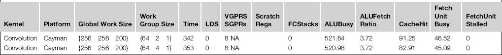
High kernel occupancy rate does not necessary indicate a more efficient execution. Take the convolution kernel as an example. The kernel occupancy rate increases from 76.19% to 95.24% while we increase the workgroup size from {64 2 1} to {64 4 1}. But the CacheHit and ALU utilization ratio reduced from 91.25% and 21.64% to 82.91% and 20.98%, respectively. As a result, the kernel execution time increases from 342 to 353 ms as shown in Table 14.2 created with numbers collected through the GPU performance counter in APP Profiler.
Table 14.2 Comparison of different workgroup sizes for the convolution kernel. Based on values obtained from APP Profiler.
Impact of VGPR and LDS
If a kernel is limited by register usage and not by LDS usage, then it is possible that moving some data into LDS will shift that limit. If a balance can be found between LDS use and registers such that register data is moved into LDS in such a way that the register count is lowered but LDS does not become a more severe limit on occupancy, then this could be a winning strategy. The same under some circumstances may be true of moving data into global memory.
However, care must be taken while making this change. Not only may LDS become the limiting factor on kernel occupancy, but accessing LDS is slower than accessing registers. Even if occupancy improves, performance may drop because the compute unit is executing more, or slower, instructions to compute the same result. This is even more true if global memory were to be used to reduce register count: this is exactly the situation we see with register spilling.
This section we show the impact of reducing kernel VGPR usage by moving some data storage to LDS to increase the kernel occupancy and improve the performance. Eigen decomposition of the Hessian matrix at each voxel of the image is used to illustrate this. The basic implementation of the eigenanalysis kernel is inserted below:
int4 coord = (int4)(get_global_id(0), get_global_id(1), get_global_id(2), 0);
value = read_imagef(h1, imageSampler,
(int4)(coord.x, coord.y, coord.z, 0));
value = read_imagef(h2, imageSampler,
(int4)(coord.x, coord.y, coord.z, 0));
matrix[1] = matrix[3] = value.x;
value = read_imagef(h3, imageSampler,
(int4)(coord.x, coord.y, coord.z, 0));
matrix[2] = matrix[6] = value.x;
value = read_imagef(h4, imageSampler,
(int4)(coord.x, coord.y, coord.z, 0));
value = read_imagef(h5, imageSampler,
(int4)(coord.x, coord.y, coord.z, 0));
matrix[5] = matrix[7] = value.x;
value = read_imagef(h6, imageSampler,
(int4)(coord.x, coord.y, coord.z, 0));
EigenDecomposition(eigenvalue, eigenvector, matrix, 3);
(float4)(eigenvalue[0], 0.0f, 0.0f, 0.0f));
(float4)(eigenvalue[1], 0.0f, 0.0f, 0.0f));
In this implementation, each eigenanalysis kernel consumes 41 GPRs, with no LDS used. Profiling with APP Profiler, we can see that this high usage of the VGPR resource limits the number of wavefronts that can be deployed to 6. As a result, the estimated occupancy ratio is 29.57%. By allocating the storage for the array matrix in LDS as shown in the following code example, the vector GPR usage per work item is reduced to 15, with LDS usage reported at 4.5K, and the number of active wavefronts 14. Consequently, the estimated occupancy ratio increases substantially to 66.67%. The kernel runtime dropped from 180 to 93 ms on average on Cayman.
(reqd_work_group_size(GROUP_SIZEx, GROUP_SIZEy, 1)))
int4 coord = (int4)(get_global_id(0), get_global_id(1), get_global_id(2), 0);
int localCoord = get_local_id(0);
The table below shows the profiler summary of the execution time of the final implementation with five different scales. These data are collected on a Radeon™ HD6970 GPU with five scales ranging from 0.5 to 4 mm and an image size of 256 × 256 × 200.

Power and performance analysis
We test the optimized application on a Trinity (A10-5800K) platform in three formats: a single-threaded CPU version, a multithreaded CPU version, and the GPU-based version. Using the AMD Graphics Manager software on the Trinity APU, we can collect the power consumption number at a fixed time interval on each device. In this case, two CPU modules (core pairs) listed as “CU” in the table and the GPU. In this test, power samples are collected at 100-ms time intervals and seven different scales for identifying vessel structure are used to increase the amount of samples collected for a more accurate analysis. Each row in the table below shows the average power consumption for each device and the total power consumption and execution time measured. Using this data, we calculate the total energy consumption. Note that despite the fact that all other applications are switched off, this approach still measures the whole system’s power consumption, not just the running application. However, it is the easiest way to get an estimated analysis without extra hardware. Using the single-threaded CPU version as baseline, we can derive the performance and energy improvement for a multithreaded CPU version and GPU-based one. We perform a similar comparison with the multithreaded CPU as baseline in the third table. In total, we observe that, despite the GPU being powered down while not in use, the energy consumption of executing the application on GPU is significantly lower than the MT-CPU one.


Conclusion
In this chapter, we showed how some of the profiling tools in the AMD APP SDK can be used to analyze and hence help optimize kernel performance. We applied runtime profiling and static analysis to a real-image analysis application to help optimize performance using OpenCL. Of course, in writing this chapter, we had to select a consistent set of tools, and in this case, to match the hardware example chapter and to make chapters link together, we choose the AMD tools. Similar data and optimizations are, of course, necessary on other architectures, and NVIDIA, Intel, and other vendors provide their own, often excellent, tools to achieve similar goals.
References
1. Frangi, A. F. (2001). Three-Dimensional Model-Based Analysis of Vascular and Cardiac Images. PhD thesis, University Medical Center Utrecht, The Netherlands.
2. Lorenz C, Carlsen I-C, Buzug TM, Fassnacht C, Weese J. Multi-scale line segmentation with automatic estimation of width, contrast and tangential direction in 2D and 3D medical images. In: Proceedings of the First Joint Conference on Computer Vision, Virtual Reality and Robotics in Medicine and Medial Robotics and Computer-Assisted Surgery. 1997:233–242.
3. Olabarriaga SD, Breeuwer M, Niessen W. Evaluation of Hessian-based filters to enhance the axis of coronary arteries in CT images. In: Computer Assisted Radiology and Surgery. 2003:1191–1196. International Congress Series Vol. 1256.
4. Sato Y, Shiraga N, Atsumi H, et al. Three-dimensional multi-scale line filter for segmentation and visualization of curvilinear structures in medical images. Medical Image Analysis. 1998;2(2):143–168.
5. Zhang, D. P. (2010). Coronary Artery Segmentation and Motion Modeling. PhD thesis, Imperial College London, UK.