5
Eternal Triangles
Trigonometry and logarithms

Euclidean geometry is based on triangles, mainly because every polygon can be built from triangles, and most other interesting shapes, such as circles and ellipses, can be approximated by polygons. The metric properties of triangles – those that can be measured, such as the lengths of sides, the sizes of angles or the total area – are related by a variety of formulas, many of them elegant. The practical use of these formulas, which are extremely useful in navigation and surveying, required the development of trigonometry, which basically means ‘measuring triangles’.
Trigonometry
Trigonometry spawned a number of special function – mathematical rules for calculating one quantity from another. These functions go by names like sine, cosine and tangent. The trigonometric functions turned out to be of vital importance for the whole of mathematics, not just for measuring triangles.
Trigonometry is one of the most widely used mathematical techniques, involved in everything from surveying to navigation to GPS satellite systems in cars. Its use in science and technology is so common that it usually goes unnoticed, as befits any universal tool. Historically, it was closely associated with logarithms, a clever method for converting multiplications (which are hard) into additions (which are easier). The main ideas appeared between about 1400 and 1600, though with a lengthy prehistory and plenty of later embellishments, and the notation is still evolving.
‘Humanity owes a great deal to these dedicated and dogged pioneers.’
In this chapter we’ll take a look at the basic topics: trigonometric functions, the exponential function and the logarithm. We also consider a few applications, old and new. Many of the older applications are computational techniques, which have mostly become obsolete now that computers are widespread. Hardly anyone now uses logarithms to do multiplication, for instance. No one uses tables at all, now that computers can rapidly calculate the values of functions to high precision. But when logarithms were first invented, it was the numerical tables of them that made them useful, especially in areas like astronomy, where long and complicated numerical calculations were necessary. And the compilers of the tables had to spend years – decades – of their lives doing the sums. Humanity owes a great deal to these dedicated and dogged pioneers.
The origins of trigonometry
The basic problem addressed by trigonometry is the calculation of properties of a triangle – lengths of sides, sizes of angles – from other such properties. It is much easier to describe the early history of trigonometry if we first summarize the main features of modern trigonometry, which is mostly a reworking in 18th century notation of topics that go right back to the Greeks, if not earlier. This summary provides a framework within which we can describe the ideas of the ancients, without getting tangled up in obscure and eventually obsolete concepts.
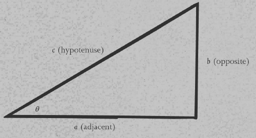
Trigonometry relies on a number of special functions, of which the most basic are the sine, cosine and tangent. These functions apply to an angle, traditionally represented by the Greek letter θ (theta). They can be defined in terms of a right triangle, whose three sides a, b, c are called the adjacent side, the opposite side and the hypotenuse.
Then:
The sine of theta is | sin θ = b/c |
The cosine of theta is | cos θ = a/c |
The tangent of theta is | tan θ = b/a |
As it stands, the values of these three functions, for any given angle θ, are determined by the geometry of the triangle. (The same angle may occur in triangles of different sizes, but the geometry of similar triangles implies that the stated ratios are independent of size.) However, once these functions have been calculated and tabulated, they can be used to solve (calculate all the sides and angles of) the triangle from the value of.
The three functions are related by a number of beautiful formulas. In particular, Pythagoras’s Theorem implies that
sin2θ + cos2θ = 1
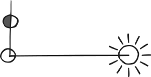
Trigonometry seems to have originated in astronomy, where it is relatively easy to measure angles, but difficult to measure the vast distances. The Greek astronomer Aristarchus, in a work of around 260 BC, On the Sizes and Distances of the Sun and Moon, deduced that the Sun lies between 18 and 20 times as far from the Earth as the Moon does. (The correct figure is closer to 400, but Eudoxus and Phidias had argued for 10.) His reasoning was that when the Moon is half full, the angle between the directions from the observer to the Sun and the Moon is about 87° (in modern units). Using properties of triangles that amount to trigonometric estimates, he deduced (in modern notation) that sin 3° lies between 1/18 and 1/20, leading to his estimate of the ratio of the distances to the Sun and the Moon. The method was right, but the observation was inaccurate; the correct angle is 89.8°.
The first trigonometric tables were derived by Hipparchus around 150 BC. Instead of the modern sine function, he used a closely related quantity, which from the geometric point of view was equally natural. Imagine a circle, with two radial lines meeting at an angle θ. The points where these lines cut the circle can be joined by a straight line, called a chord. They can also be thought of as the end points of a curved arc of the circle. Hipparchus drew up a table relating arc and chord length for a range of angles. If the circle has radius 1, then the arc length is equal to θ when this angle is measured in units known as radians. Some easy geometry shows that the chord length in modern notation is 2sin ![]() . So Hipparchus’s calculation is very closely related to a table of sines, even though it was not presented in that way.
. So Hipparchus’s calculation is very closely related to a table of sines, even though it was not presented in that way.
Relation between the Sun, Moon, and Earth when the Moon is half full
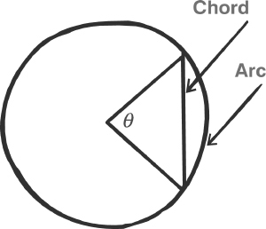
Arc and chord corresponding to an angle θ
Astronomy
Remarkably, early work in trigonometry was more complicated than most of what is taught in schools today, again because of the needs of astronomy (and, later, navigation). The natural space to work in was not the plane, but the sphere. Heavenly objects can be thought of as lying on an imaginary sphere, the celestial sphere. Effectively, the sky looks like the inside of a gigantic sphere surrounding the observer, and the heavenly bodies are so distant that they appear to lie on this sphere.
Astronomical calculations, in consequence, refer to the geometry of a sphere, not that of a plane. The requirements are therefore not plane geometry and trigonometry, but spherical geometry and trigonometry. One of the earliest works in this area is Menelaus’s Sphaerica of about AD100. A sample theorem, one that has no analogue in Euclidean geometry, is this: if two triangles have the same angles as each other, then they are congruent – they have the same size and shape. (In the Euclidean case, they are similar – same shape but possibly different sizes.) In spherical geometry, the angles of a triangle do not add up to 180°, as they do in the plane. For example, a triangle whose vertices lie at the North Pole and at two points on the equator separated by 90° clearly has all three angles equal to a right angle, so the sum is 270°. Roughly speaking, the bigger the triangle becomes, the bigger its angle-sum becomes. In fact, this sum, minus 180°, is proportional to the triangle’s total area.
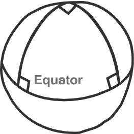
North Pole
These examples make it clear that spherical geometry has its own characteristic and novel features. The same goes for spherical trigonometry, but the basic quantities are still the standard trigonometric functions. Only the formulas change.
Ptolemy
By far and above the most important trigonometry text of antiquity was the Mathematical Syntaxis of Ptolemy of Alexandria, which dates to about AD150. It is better known as the Almagest, an Arabic term meaning ‘the greatest’. It included trigonometric tables, again stated in terms of chords, together with the methods used to calculate them, and a catalogue of star positions on the celestial sphere. An essential feature of the computational method was Ptolemy’s Theorem which states that if ABCD is a cyclic quadrilateral (one whose vertices lie on a circle) then
AB × CD + BC × DA = AC × BD

Cyclic quadrilateral and its diagonals
(the sum of the products of opposite pairs of sides is equal to the product of the diagonals).
A modern interpretation of this fact is the remarkable pair of formulas
sin (θ + φ) = sin θ cos φ + cos θ sin φ
cos (θ + φ) = cos θ cos φ – sin θ sin φ
The main point about these formulas is that if you know the sines and cosines of two angles, then you can easily work the sines and cosines out for the sum of those angles. So, starting with (say) sin 1° and cos 1°, you can deduce sin 2° and cos 1° by taking θ = φ = 1°. Then you can deduce sin 3° and cos 3° by taking θ = 1°, φ = 2°, and so on. You had to know how to start, but after that, all you needed was arithmetic – rather a lot of it, but nothing more complicated.
Getting started was easier than it might seem, requiring arithmetic and square roots. Using the obvious fact that θ/2 + θ/2 = θ, Ptolemy’s Theorem implies that
![]()
Starting from cos 90° = 0, you can repeatedly halve the angle, obtaining sines and cosines of angles as small as you please. (Ptolemy used ¼°.) Then you can work back up through all integer multiples of that small angle. In short, starting with a few general trigonometric formulas, suitably applied, and a few simple values for specific angles you can work out values for pretty much any angle you want. It was an extraordinary tour de force, and it put astronomers in business for well over a thousand years.
A final noteworthy feature of the Almagest s how it handled the orbits of the planets. Anyone who watches the night sky regularly quickly discovers that the planets wander against the background of fixed stars, and that the paths they follow seem rather complicated, sometimes moving backwards, or travelling in elongated loops.
Eudoxus, responding to a request from Plato, had found a way to represent these complex motions in terms of revolving spheres mounted on other spheres. This idea was simplified by Apollonius and Hipparchus, to use epicycles – circles whose centres move along other circles, and so on. Ptolemy refined the system of epicycles, so that it provided a very accurate model of the planetary motions.
Early trigonometry
Early trigonometric concepts appear in the writings of Hindu mathematicians and astronomers: Varahamihira’s Pancha Siddhanta of 500, Brahmagupta’s Brahma Sputa Siddhanta of 628 and the more detailed Siddhanta Siromani of Bhaskaracharya in 1150.
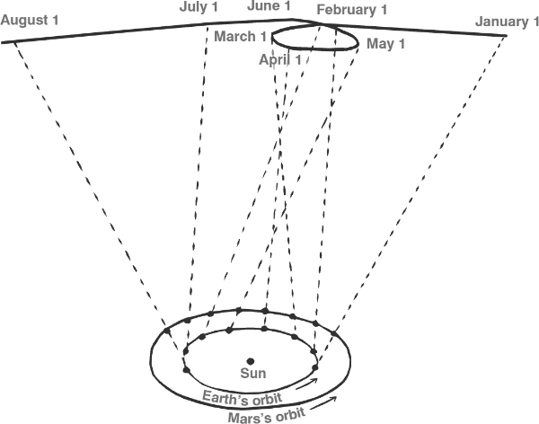
Motion of Mars as viewed from the Earth
Indian mathematicians generally used the half-chord, or jya-ardha, which is in effect the modern sine. Varahamihira calculated this function for 24 integer-multiples of 3°45, up to 90°. Around 600, in the Maha Bhaskariya, Bhaskara gave a useful approximate formula for the sine of an acute angle, which he credited to Aryabhata. These authors derived a number of basic trigonometric formulas.
The Arabian mathematician Nasîr-Eddin’s Treatise on the Quadrilateral combined plane and spherical geometry into a single unified development, and gave several basic formulas for spherical triangles. He treated the topic mathematically, rather than as a part of astronomy. But his work went unnoticed in the West until about 1450.
‘Early trigonometric concepts appear in the writings of Hindu mathematicians and astronomers.’
Because of the link with astronomy, almost all trigonometry was spherical until 1450. In particular, surveying – today a major user of trigonometry – was carried out using empirical methods, codified by the Romans. But in the mid-15th century, plane trigonometry began to come into its own, initially in the north German Hanseatic League. The League was in control of most trade, and consequently was rich and influential. And it needed improved navigational methods, along with improved timekeeping and practical uses of astronomical observations.
A key figure was Johannes Müller, usually known as Regiomontanus. He was a pupil of George Peuerbach, who began working on a new corrected version of the Almagest. In 1471, financed by his patron Bernard Walther, he computed a new table of sines and a table of tangents.
Other prominent mathematicians of the 15th and 16th centuries computed their own trigonometric tables, often to extreme accuracy. George Joachim Rhaeticus calculated sines for a circle of radius 1015 – effectively, tables accurate to 15 decimal places, but multiplying all numbers by 1015 to get integers – for all multiples of one second of arc. He stated the law of sines for spherical triangles
![]()
and the law of cosines
cos a = cos b cos c + sin b sin c cos A
in his De Triangulis, written in 1462–3 but not published until 1533. Here A, B, C are the angles of the triangle, and a, b, c are its sides – measured by the angles they determine at the centre of the sphere.
Vieta wrote widely on trigonometry, with his first book on the topic being the Canon Mathematicus of 1579. He collected and systematized various methods for solving triangles, that is, calculating all sides and angles from some subset of information. He invented new trigonometric identities, among them some interesting expressions for sines and cosines of integer multiples of θ in terms of the sine and cosine of θ.
Logarithms
The second theme of this chapter is one of the most important functions in mathematics: the logarithm, log x. Initially, the logarithm was important because it satisfies the equation
log xy = log x + log y
and can therefore be used to convert multiplications (which are cumbersome) into additions (which are simpler and quicker). To multiply two numbers x and y, first find their logarithms, add them and then find the number whose logarithm is that result (its antilogarithm). This is the product xy.
Once mathematicians had calculated tables of logarithms, they could be used by anyone who understood the method. From the 17th century until the mid-20th, virtually all scientific calculations, especially astronomical ones, employed logarithms. From the 1960s onwards, however, electronic calculators and computers rendered logarithms obsolete for purposes of calculation. But the concept remained vital to mathematics, because logarithms had found fundamental roles in many parts of mathematics, including calculus and complex analysis. Also many physical and biological processes involve logarithmic behaviour.
Nowadays we approach logarithms by thinking of them as the reverse of exponentials. Using logarithms to base 10, which are a natural choice for decimal notation, we say that x is the logarithm of y if y = 10x. For example, since 103 = 1000, the logarithm of 1000 (to base 10) is 3. The basic property of logarithms follows from the exponential law
10a+b = 10a × 10b
However, in order for the logarithm to be useful, we have to be able to find a suitable x for any positive real y. Following the lead of Newton and others of his period, the main idea is that any rational power 10p/q can be defined to be the qth root of 10p. Since any real number x can be approximated arbitrarily closely by a rational number p/q, we can approximate 10x by 10p/q. This is not the most efficient way to calculate the logarithm, but it is the simplest way to prove that it exists.
Historically, the discovery of logarithms was less direct. It began with John Napier, Baron of Murchiston in Scotland. He had a lifelong interest in efficient methods for calculation, and invented Napier’s rods (or Napier’s bones), a set of marked sticks that could be used to perform multiplication quickly and reliably by simulating pen-and-paper methods. Around 1594 he started working on a more theoretical method, and his writings tell us that it took him 20 years to perfect and publish it. It seems likely that he started with geometric progressions, sequences of numbers in which each term is obtained from the previous one by multiplying by a fixed number – such as the powers of 2
Nowadays trigonometry is first developed in the plane, where the geometry is simpler and the basic principles are easier to grasp. (It is curious how often new mathematical ideas are first developed in a complicated context, and the underlying simplicities emerge much later.) There is a law of sines, and a law of cosines, for plane triangles, and it is worth a quick digression to explain these. Consider a plane triangle with angles A, B, C and sides a, b, c.
Now the law of sines takes the form
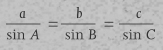
and the law of cosines is
a2 = b2 + c2 – 2bc cos A,
with companion formulas involving the other angles. We can use the law of cosines to find the angles of a triangle from its sides.
Sides and angles of a triangle
1 2 4 8 16 32 . . .
or powers of 10
1 10 100 1000 10,000 100,000 . . .
Here it had long been noticed that adding the exponents was equivalent to multiplying the powers. This was fine if you wanted to multiply two integer powers of 2, say, or two integer powers of 10. But there were big gaps between these numbers, and powers of 2 or 10 seemed not to help much when it came to problems like 57.681 × 29.443, say.
Napierian logarithms
While the good Baron was trying to somehow fill in the gaps in geometric progressions, the physician to King James VI of Scotland, James Craig, told Napier about a discovery that was in widespread use in Denmark, with the ungainly name prosthapheiresis. This referred to any process that converted products into sums. The main method in practical use was based on a formula discovered by Vieta:
![]()
If you had tables of sines and cosines, you could use this formula to convert a product into a sum. It was messy, but it was still quicker than multiplying the numbers directly.
Napier seized on the idea, and found a major improvement. He formed a geometric series with a common ratio very close to 1. That is, in place of the powers of 2 or powers of 10, you should use powers of, say, 1.0000000001. Successive powers of such a number are very closely spaced, which gets rid of those annoying gaps. For some reason Napier chose a ratio slightly less than 1, namely 0.9999999. So his geometric sequence ran backwards from a large number to successively smaller ones. In fact, he started with 10,000,000 and then multiplied this by successive powers of 0.9999999. If we write Naplog x for Napier’s logarithm of x, it has the curious feature that
‘Napier seized on the idea, and found a major improvement.’
Naplog 10,000,000 = 0
Naplog 9,999,999 = 1
and so on. The Napierian logarithm, Naplog x, satisfies the equation
Naplog(107xy) = Naplog(x) + Naplog(y)
You can use this for calculation, because it is easy to multiply or divide by a power of 10, but it lacks elegance. It is, however, much better than Vieta’s trigonometric formula.
Base ten logarithms
The next improvement came when Henry Briggs, the first Savilian professor of geometry at the University of Oxford, visited Napier. Briggs suggested replacing Napier’s concept by a simpler one: the (base ten) logarithm, L = log10 x, which satisfies the condition
x = 10L.
Now
log10 xy = log10 x + log10 y
and everything is easy. To find xy, add the logarithms of x and y and then find the antilogarithm of the result.
Before these ideas could be disseminated, Napier died; the year was 1617, and his description of his calculating rods, Rhabdologia, had just been published. His original method for calculating logarithms, the Mirifici Logarithmorum Canonis Constructio, appeared two years later. Briggs took up the task of computing a table of Briggsian (base 10, or common) logarithms. He did this by starting from log1010 = 1 and taking successive square roots. In 1617 he published Logarithmorum Chilias Prima, the logarithms of the integers from 1 to 1000, stated to 14 decimal places. His 1624 Arithmetic Logarithmica tabulated common logarithms of numbers from 1 to 20,000 and from 90,000 to 100,000, also to 14 places.
What trigonometry did for them
Ptolemy’s Almagest formed the basis of all studies of planetary motion prior to Johannes Kepler’s discovery that orbits are elliptical. The observed movements of a planet are complicated by the relative motion of the Earth, which was not recognized in Ptolemy’s time. Even if planets moved at uniform speed in circles, the Earth’s motion round the Sun would effectively require a combination of two different circular motions, and an accurate model has to be distinctly more complicated than Ptolemy’s model. Ptolemy’s scheme of epicycles combines circular motions by making the centre of one circle revolve around another circle. This circle can itself revolve round a third circle, and so on. The geometry of uniform circular motion naturally involves trigonometric functions, and later astronomers used these for calculations of orbits.

An epicycle. Planet P revolves uniformly around point D, which in turn revolves uniformly around point C.
The idea snowballed. John Speidell worked out logarithms of trigonometric functions (such as log sin x) published as New Logarithmes in 1619. The Swiss clockmaker Jobst Bürgi published his own work on logarithms in 1620, and may well have possessed the basic idea in 1588, well before Napier. But the historical development of mathematics depends on what people publish – in the original sense of make public – and ideas that remain private have no influence on anyone else. So credit, probably rightly, has to go to those people who put their ideas into print, or at least into widely circulated letters. (The exception is people who put the ideas of others into print without due credit. This is generally beyond the pale.)
The number e
Associated with Napier’s version of logarithms is one of the most important numbers in mathematics, now denoted by the letter e. Its value is roughly 2.7128. It arises if we try to from logarithms by starting from a geometric series whose common ratio is very slightly larger than 1. This leads to the expression (1 + 1/n)n, where n is a very large integer, and the larger n becomes, the closer this expression is to one special number, which we denote by e.
This formula suggests that there is a natural base for logarithms, and it is neither 10 nor 2, but e. The natural logarithm of x is whichever number y satisfies the condition x = ey. In today’s mathematics the natural logarithm is written y = log x. Sometimes the base e is made explicit, as y = loge x, but this notation is mainly restricted to school mathematics, because in advanced mathematics and science the only logarithm of importance is the natural logarithm. Base ten logarithms are best for calculations in decimal notation, but natural logarithms are more fundamental mathematically.
The expression ex is called the exponential of x, and it is one of the most important concepts in the whole of mathematics. The number e is one of those strange special numbers that appear in mathematics, and have major significance. Another such number is π. These two numbers are the tip of an iceberg – there are many others. They are also arguably the most important of the special numbers because they crop up all over the mathematical landscape.
Where would we be without them?
It would be difficult to underestimate the debt that we owe to those far-seeing individuals who invented logarithms and trigonometry, and spent years calculating the first numerical tables. Their efforts paved the way to a quantitative scientific understanding of the natural world, and enabled worldwide travel and commerce by improving navigation and map-making. The basic techniques of surveying rely on trigonometric calculations. Even today, when surveying equipment uses lasers and the calculations are done on a custom-built electronic chip, the concepts that the laser and the chip embody are direct descendants of the trigonometry that intrigued the mathematicians of ancient India and Arabia.
Logarithms made it possible for scientists to do multiplication quickly and accurately. Twenty years of effort on a book of tables, by one mathematician, saved tens of thousands of man-years of work later on. It then became possible to carry out scientific analyses using pen and paper that would otherwise have been too time-consuming. Science could never have advanced without some such method. The benefits of such a simple idea have been incalculable.
Trigonometry is fundamental to surveying anything from building sites to continents. It is relatively easy to measure angles to high accuracy, but harder to measure distances, especially on difficult terrain. Surveyors therefore begin by making a careful measurement of one length, the baseline, that is, the distance between two specific locations. They then form a network of triangles, and use the measured angles, plus trigonometry, to calculate the sides of these triangles. In this manner, an accurate map of the entire area concerned can be constructed. This process is known as triangulation. To check its accuracy, a second distance measurement can be made once the triangulation is complete.
The figure here shows an early example, a famous survey carried out in South Africa in 1751 by the great astronomer Abbé Nicolas Louis de Lacaille. His main aim was to catalogue the stars of the southern skies, but to do this accurately he first had to measure the arc of a suitable line of longitude. To do this, he developed a triangulation to the north of Cape Town.
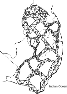
LaCaille’s triangulation of South Africa
His result suggested that the curvature of the earth is less in southern latitudes than in northern ones, a surprising deduction which was verified by later measurements. The Earth is slightly pear-shaped. His cataloguing activities were so successful that he named 15 of the 88 constellations now recognized, having observed more than 10,000 stars using a small refracting telescope.