6 Curves and Coordinates

Geometry is algebra is geometry

Although it is usual to classify mathematics into separate areas, such as arithmetic, algebra, geometry and so on, this classification owes more to human convenience than the subject’s true structure. In mathematics, there are no hard and fast boundaries between apparently distinct areas, and problems that seem to belong to one area may be solved using methods from another. In fact, the greatest breakthroughs often hinge upon making some unexpected connection between previously distinct topics.

Fermat

Greek mathematics has traces of such connections, with links between Pythagoras’s Theorem and irrational numbers, and Archimedes’s use of mechanical analogies to find the volume of the sphere. The true extent and influence of such cross-fertilization became undeniable in a short period ten years either side of 1630. During that brief time, two of the world’s greatest mathematicians discovered a remarkable connection between algebra and geometry. In fact, they showed that each of these areas can be converted into the other by using coordinates. Everything in Euclid, and the work of his successors, can be reduced to algebraic calculations. Conversely, everything in algebra can be interpreted in terms of the geometry of curves and surfaces.

It might seem that such connections render one or other area superfluous. If all geometry can be replaced by algebra, why do we need geometry? The answer is that each area has its own characteristic point of view, which can on occasion be very penetrating and powerful. Sometimes it is best to think geometrically, and sometimes algebraic thinking is superior.

The first person to describe coordinates was Pierre de Fermat. Fermat is best known for his work in number theory, but he also studied many other areas of mathematics, including probability, geometry and applications to optics. Around 1620, Fermat was trying to understand the geometry of curves, and he started by reconstructing, from what little information was available, a lost book by Apollonius called On Plane Loci. Having done this, Fermat embarked upon his own investigations, writing them up in 1629 but not publishing them until 50 years later, as Introduction to Plane and Solid Loci. By so doing, he discovered the advantages of rephrasing geometrical concepts in algebraic terms.

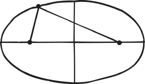
Focal property of the ellipse

Locus, plural loci, is an obsolete term today, but it was common even in 1960. It arises when we seek all points in the plane or space that satisfy particular geometric conditions. For example, we might ask for the locus of all points whose distances from two other fixed points always add up to the same total. This locus turns out to be an ellipse with the two points as its foci. This property of the ellipse was known to the Greeks.

Fermat noticed a general principle: if the conditions imposed on the point can be expressed as a single equation involving two unknowns, the corresponding locus is a curve – or a straight line, which we consider to be a special kind of curve to avoid making needless distinctions. He illustrated this principle by a diagram in which the two unknown quantities A and E are represented as distances in two distinct directions.

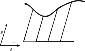
Fermat’s approach to coordinates

He then listed some special types of equation connecting A and E, and explained what curves they represent. For instance, if A² = 1 + E² then the locus concerned is a hyperbola.

‘Fermat introduced oblique axes in the plane.’

In modern terms, Fermat introduced oblique axes in the plane (oblique meaning that they do not necessarily cross at right angles). The variables A and E are the two coordinates, which we would call x and y, of any given point with respect to these axes. So Fermat’s principle effectively states that any equation in two-coordinate variables defines a curve, and his examples tell us what kind of equations correspond to what kind of curve, drawing on the standard curves known to the Greeks.

Descartes

The modern notion of coordinates came to fruition in the work of Descartes. In everyday life, we are familiar with spaces of two and three dimensions, and it takes a major effort of imagination for us to contemplate other possibilities. Our visual system presents the outside world to each eye as a two-dimensional image – like the picture on a TV screen. Slightly different images from each eye are combined by the brain to provide a sense of depth, through which we perceive the surrounding world as having three dimensions.

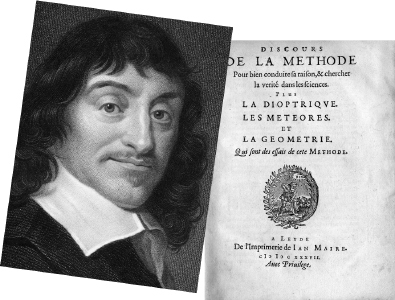
The key to multidimensional spaces is the idea of a coordinate system, which was introduced by Descartes in an appendix La Géometrie to his book Discours de la Méthode. His idea is that the geometry of the plane can be reinterpreted in algebraic terms. His approach is essentially the same as Fermat’s. Choose some point in the plane and call it the origin. Draw two axes, lines that pass through the origin and meet at right angles. Label one axis with the symbol x and the other with the symbol y. Then any point P in the plane is determined by the pair of distances (x, y), which tells us how far the point is from the origin when measured parallel to the x- and y-axes, respectively.

For example, on a map, x might be the distance east of the origin (with negative numbers representing distances to the west), whereas y might be the distance north of the origin (with negative numbers representing distances to the south).

René Descartes

1596–1650

Descartes first began to study mathematics in 1618, as a student of the Dutch scientist Isaac Beeckman. He left Holland to travel through Europe, and joined the Bavarian army in 1619. He continued to travel between 1620 and 1628, visiting Bohemia, Hungary, Germany, Holland, France and Italy. He met Mersenne in Paris in 1622, and corresponded regularly with him thereafter, which kept him in touch with most of the leading scholars of the period.

In 1628 Descartes settled in Holland, and started his first book Le Monde, ou Traité de la Lumière, on the physics of light. Publication was delayed when Descartes heard of Galileo Galilei’s house arrest, and Descartes got cold feet. The book was published, in an incomplete form, after his death. Instead, he developed his ideas on logical thinking into a major work published in 1637: Discours de la Méthode. The book had three appendices: La Dioptrique, Les Météores and La Géométrie.

His most ambitious book, Principia Philosophiae, was published in 1644. It was divided into four parts: Principles of Human Knowledge, Principles of Material Things, The Visible World and The Earth. It was an attempt to provide a unified mathematical foundation for the entire physical universe, reducing everything in nature to mechanics.

In 1649 Descartes went to Sweden, to act as tutor to Queen Christina. The Queen was an early riser, whereas Descartes habitually rose at 11 o’clock. Tutoring the Queen in mathematics at 5 o’clock every morning, in a cold climate, imposed a considerable strain on Descartes’s health. After a few months, he died of pneumonia.

Coordinates work in three-dimensional space too, but now two numbers are not sufficient to locate a point. However, three numbers are. As well as the distances east–west and north–south, we need to know how far the point is above or below the origin. Usually we use a positive number for distances above, and a negative one for distances below. Coordinates in space take the form (x, y, z).

This is why the plane is said to be two-dimensional, whereas space is three-dimensional. The number of dimensions is given by how many numbers we need to specify a point.

In three-dimensional space, a single equation involving x, y and z usually defines a surface. For example, x² + y² + z² = 1 states that the point (x, y, z) is always a distance 1 unit from the origin, which implies that it lies on the unit sphere whose centre is the origin.

Notice that the word ‘dimension’ is not actually defined here in its own right. We do not find the number of dimensions of a space by finding some things called dimensions and then counting them. Instead, we work out how many numbers are needed to specify where a location in the space is, and that is the number of dimensions.

Cartesian coordinates

Cartesian coordinate geometry reveals an algebraic unity behind the conic sections – curves that the Greeks had constructed as sections of a double cone. Algebraically, it turns out that the conic sections are the next simplest curves after straight lines. A straight line corresponds to a linear equation

ax + by + c = 0

with constants a, b, c. A conic section corresponds to a quadratic equation

ax² + bxy + cy² + dx + ey + f = 0

with constants a, b, c, d, e, f. Descartes stated this fact, but did not provide a proof. However, he did study a special case, based on a theorem due to Pappus which characterized conic sections, and he showed that in this case the resulting equation is quadratic.

He went on to consider equations of higher degree, defining curves more complex than most of those arising in classical Greek geometry. A typical example is the folium of Descartes, with equation

x³ + y³ – 3axy = 0

which forms a loop with two ends that tend to infinity.

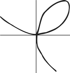
The folium of Descartes

Perhaps the most important contribution made by the concept of coordinates occurred here: Descartes moved away from the Greek view of curves as things that are constructed by specific geometric means, and saw them as the visual aspect of any algebraic formula. As Isaac Newton remarked in 1707, ‘The moderns advancing yet much further [than the Greeks] have received into geometry all lines that can be expressed by equations’.

Later scholars invented numerous variations on the Cartesian coordinate system. In a letter of 1643 Fermat took up Descartes’s ideas and extended them to three dimensions. Here he mentioned surfaces such as ellipsoids and paraboloids, which are determined by quadratic equations in the three variables x, y, z. An influential contribution was the introduction of polar coordinates by Jakob Bernoulli in 1691. He used an angle θ and a distance r to determine points in the plane instead of a pair of axes. Now the coordinates are (r, θ).

Again, equations in these variables specify curves. But now, simple equations can specify curves that would become very complicated in Cartesian coordinates. For example the equation r = θ corresponds to a spiral, of the kind known as an Archimedean spiral.

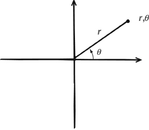
Polar coordinates

Functions

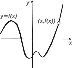
An important application of coordinates in mathematics is a method to represent functions graphically.

A function is not a number, but a recipe that starts from some number and calculates an associated number. The recipe involved is often stated as a formula, which assigns to each number, x (possibly in some limited range), another number, f(x).

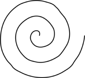
Archimedean spiral

For example, the square root function is defined by the rule f(x) = , that is, take the square root of the given number. This recipe requires x to be positive. Similarly the square function is defined by f(x) = x², and this time there is no restriction on x.

Which Bernoulli Did What?

A Bernoulli Checklist

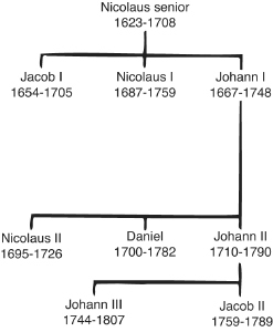
The Swiss Bernoulli family had a huge influence on the development of mathematics. Over some four generations they produced significant mathematics, both pure and applied. Often described as a mathematical mafia, the Bernoullis typically started out in careers like law, medicine or the church, but eventually reverted to type and became mathematicians, either professional or amateur.

Many different mathematical concepts bear the name Bernoulli. This is not always the same Bernoulli. Rather than providing biographical details about them, here is a summary of who did what.

Jacob I (1654–1705)

Polar coordinates, formula for the radius of curvature of a plane curve. Special curves, such as the catenary and lemniscate. Proved that an isochrone (a curve along which a body will fall with uniform vertical velocity) is an inverted cycloid. Discussed isoperimetric figures, having the shortest length under various conditions, a topic that later led to the calculus of variations. Early student of probability and author of the first book on the topic, Ars Conjectandi. Asked for a logarithmic spiral to be engraved on his tombstone, along with the inscription Eadem mutata resurgo (I shall arise the same though changed).

Johann I (1667–1748)

Developed the calculus and promoted it in Europe. The Marquis de L’Hôpital put Johann’s work into the first calculus textbook. ‘L’Hôpital’s rule’ for evaluating limits reducing to ⁰/₀ is due to Johann. Wrote on optics (reflection and refraction), orthogonal trajectories of families of curves, lengths of curves and evaluation of areas by series, analytical trigonometry and the exponential function. Brachistochrone (curve of quickest descent), length of cycloid.

Nicolaus I (1687–1759)

Held Galileo’s chair of mathematics at Padua. Wrote on geometry and differential equations. Later, taught logic and law. A gifted but not very productive mathematician. Corresponded with Leibniz, Euler and others – his main achievements are scattered among 560 items of correspondence. Formulated the St Petersburg Paradox in probability.

Criticized Euler’s indiscriminate use of divergent series. Assisted in publication of Jacob Bernoulli’s Ars Conjectandi. Supported Leibniz in his controversy with Newton.

Nicolaus II (1695–1726)

Called to the St. Petersburg Academy, died by drowning eight months later. Discussed the St Petersburg Paradox with Daniel.

Daniel (1700–1782)

Most famous of Johann’s three sons. Worked on probability, astronomy, physics and hydrodynamics. His Hydrodynamica of 1738 contains Bernoulli’s principle about the relation between pressure and velocity. Wrote on tides, the kinetic theory of gases and vibrating strings. Pioneer in partial differential equations.

Johann II (1710–1790)

Youngest of Johann’s three sons. Studied law but became professor of mathematics at Basel. Worked on the mathematical theory of heat and light.

Johann III (1744–1807)

Like his father, studied law but then turned to mathematics. Called to the Berlin Academy at age 19. Wrote on astronomy, chance and recurring decimals.

Jacob II (1759–1789)

Important works on elasticity, hydrostatics, and ballistics.

We can picture a function geometrically by defining the y-coordinate, for a given value of x, by y = f(x). This equation states a relationship between the two coordinates, and therefore determines a curve. This curve is called the graph of the function f.

The graph of the function f(x) = x² turns out to be a parabola. That of the square root f(x) = is half a parabola, but lying on its side. More complicated functions lead to more complicated curves. The graph of the sine function y = sin x is a wiggly wave.

Graph of a function f

Coordinate geometry today

Coordinates are one of those simple ideas that has had a marked influence on everyday life. We use them everywhere, usually without noticing what we’re doing. Virtually all computer graphics employ an internal coordinate system, and the geometry that appears on the screen is dealt with algebraically. An operation as simple as rotating a digital photograph through a few degrees, to get the horizon horizontal, relies on coordinate geometry.

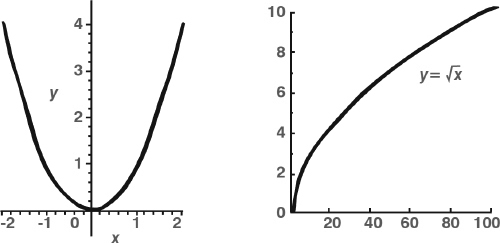
Graphs of the square and square root

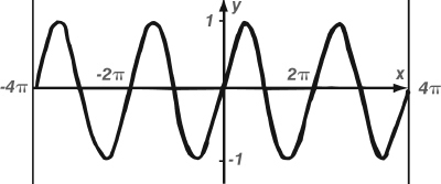
Graph of the sine function

The deeper message of coordinate geometry is about cross-connections in mathematics. Concepts whose physical realizations seem totally different may be different aspects of the same thing. Superficial appearances can be misleading. Much of the effectiveness of mathematics as a way to understand the universe stems from its ability to adapt ideas, transferring them from one area of science to another. Mathematics is the ultimate in technology transfer. And it is those cross-connections, revealed to us over the past 4000 years, that make mathematics a single, unified subject.

What coordinates did for them

Coordinate geometry can be employed on surfaces more complicated than the plane, such as the sphere. The commonest coordinates on the sphere are longitude and latitude. So map-making, and the use of maps in navigation, can be viewed as an application of coordinate geometry.

The main navigational problem for a captain was to determine the latitude and longitude of his ship. Latitude is relatively easy, because the angle of the Sun above the horizon varies with latitude and can be tabulated. Since 1730, the standard instrument for finding latitude was the sextant (now made almost obsolete by GPS). This was invented by Newton, but he did not publish it. It was independently rediscovered by the English mathematician John Hadley and the American inventor Thomas Godfrey. Previous navigators had used the astrolabe, which goes back to medieval Arabia.

Longitude is trickier. The problem was eventually solved by constructing a highly accurate clock, which was set to local time at the start of the voyage. The time of sunrise and sunset, and the movements of the Moon and stars, depend on longitude, making it possible to determine longitude by comparing local time with that on the clock. The story of John Harrison’s invention of the chronometer, which solved the problem, is famously told in Dava Sobel’s Longitude.

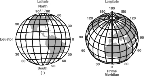
Longitude and latitude as coordinates

What coordinates do for us

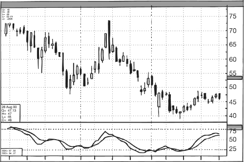
We continue to use coordinates for maps, but another common use of coordinate geometry occurs in the stock market, where the fluctuations of some price are recorded as a curve. Here the x-coordinate is time, and the y-coordinate is the price. Enormous quantities of financial and scientific data are recorded in the same way.

Stock market data represented in coordinates