9
Patterns in Nature
Formulating laws of physics

The main message in Newton’s Principia was not the specific laws of nature that he discovered and used, but the idea that such laws exist – together with evidence that the way to model nature’s laws mathematically is with differential equations. While England’s mathematicians engaged in sterile vituperation over Leibniz’s alleged (and totally fictitious) theft of Newton’s ideas about calculus, the continental mathematicians were cashing in on Newton’s great insight, making important inroads into celestial mechanics, elasticity, fluid dynamics, heat, light and sound – the core topics of mathematical physics. Many of the equations that they derived remain in use to this day, despite – or perhaps because of – the many advances in the physical sciences.
Differential equations
To begin with, mathematicians concentrated on finding explicit formulas for solutions of particular kinds of ordinary differential equation. In a way this was unfortunate, because formulas of this type usually fail to exist, so attention became focused on equations that could be solved by a formula rather than equations that genuinely described nature. A good example is the differential equation for a pendulum, which takes the form
‘. . .attention became focused on equations that could be solved by a formula. . .’
![]()
for a suitable constant k, where t is time and θ is the angle at which the pendulum hangs, with θ = 0 being vertically downwards. There is no solution of this equation in terms of classical functions (polynomial, exponential, trigonometric, logarithmic and so on). There does exist a solution using elliptic functions, invented more than a century later. However, if it is assumed that the angle is small, so we are considering a pendulum making small oscillations, then sin θ is approximately equal to θ, and the smaller θ becomes the better this approximation is. So the differential equation can be replaced by
![]()
and now there is a formula for the solution, in general,
θ = A sin kt + B cos kt
for constants A and B, determined by the initial position and angular velocity of the pendulum.
This approach has some advantages: for instance, we can quickly deduce that the period of the pendulum – the time taken to complete one swing – is 2π/k. The main disadvantage is that the solution fails when θ becomes sufficiently large (and here even 20° is large if we want an accurate answer). There is also a question of rigour: is it the case that an exact solution to an approximate equation yields an approximate solution to the exact equation? Here the answer is yes, but this was not proved until about 1900.
The second equation can be solved explicitly because it is linear – it involves only the first power of the unknown θ and its derivative, and the coefficients are constant. The prototype function for all linear differential equations is the exponential y = ex. This satisfies the equation
![]()
That is, ex is its own derivative. This property is one reason why the number e is natural. A consequence is that the derivative of the natural logarithm log x is 1/x, so the integral of 1/x is log x. Any linear differential equation with constant coefficients can be solved using exponentials and trigonometric functions (which we will see are really exponentials in disguise).
Types of differential equation
There are two types of differential equation. An ordinary differential equation (ODE) refers to an unknown function y of a single variable x, and relates various derivatives of y, such as dy/dx and d2y/dx2. The differential equations described so far have been ordinary ones. Far more difficult, but central to mathematical physics, is the concept of a partial differential equation (PDE). Such an equation refers to an unknown function y of two or more variables, such as f(x, y, t) where x and y are coordinates in the plane and t is time. The PDE relates this function to expressions in its partial derivatives with respect to each of the variables. A new notation is used to represent derivatives of some variables with respect to others, while the remainder are held fixed. Thus, ∂x/∂t indicates the rate of change of x with respect to time, while y is held constant. This is called a partial derivative – hence the term partial differential equation.
Euler introduced PDEs in 1734 and d’Alembert did some work on them in 1743, but these early investigations were isolated and special. The first big breakthrough came in 1746, when d’Alembert returned to an old problem, the vibrating violin string. John Bernoulli had discussed a finite element version of this question in 1727, considering the vibrations of a finite number of point masses spaced equally far apart along a weightless string. D’Alembert treated a continuous string, of uniform density, by applying Bernoulli’s calculations to n masses, and then letting n tend to infinity. Thus, a continuous string was in effect thought of as infinitely many infinitesimal segments of string, connected together.
Starting from Bernoulli’s results, which were based on Newton’s law of motion, and making some simplifications (for example, that the size of the vibration is small), d’Alembert was led to the PDE
![]()
where y = y(x,t) is the shape of the string at time t, as a function of the horizontal coordinate x. Here a is a constant related to the tension in the string and its density. By an ingenious argument, d’Alembert proved that the general solution of his PDE has the form
y(x, t) = f(x + at) + f(x − at)
where f is periodic, with period twice the length of the string, and f is an odd function – that is, f(−z) = −f(z). This form satisfies the natural boundary condition that the ends of the string do not move.
Wave equation
We now call d’Alembert’s PDE the wave equation, and interpret its solution as a superposition of symmetrically placed waves, one moving with velocity a and the other velocity –a (that is, travelling in the opposite direction). It has become one of the most important equations in mathematical physics, because waves arise in many different circumstances.
Euler spotted d’Alembert’s paper, and immediately tried to improve on it. In 1753 he showed that without the boundary conditions, the general solution is
y(x, t) = f(x + at) + g(x − at)
where f and g are periodic, but satisfy no other conditions. In particular, these functions can have different formulas in different ranges of x, a feature that Euler referred to as discontinuous functions, though in today’s terminology they are continuous but have discontinuous first derivatives.
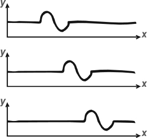
Successive snapshots of a wave travelling from left to right
In an earlier paper published in 1749 he pointed out that (for simplicity we will take the length of the string to be 1 unit) the simplest odd periodic functions are trigonometric functions
f(x) = sin x, sin 2x, sin 3x, sin 4x, . . .
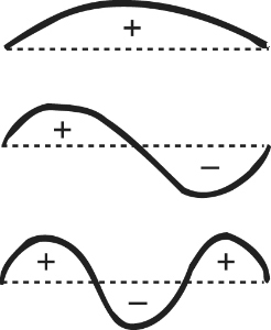
Vibrational modes of a string
and so on. These functions represent pure sinusoidal vibrations of frequencies 1, 2, 3, 4 and so on. The general solution, said Euler, is a superposition of such curves. The basic sine curve sin x is the fundamental mode of vibration, and the others are higher modes – what we now call harmonics.
Comparison of Euler’s solution of the wave equation with d’Alembert’s led to a foundational crisis. D’Alembert did not recognize the possibility of discontinuous functions in Euler’s sense. Moreover, there seemed to be a fundamental flaw in Euler’s work, because trigonometric functions are continuous, and so are all (finite) superpositions of them. Euler had not committed himself on the issue of finite superpositions versus infinite ones – in those days no one was really very rigorous about such matters, having yet to learn the hard way that it matters. Now the failure to make such a distinction was causing serious trouble. The controversy simmered until later work by Fourier caused it to boil over.
‘The ancient Greeks knew that a vibrating string can produce many different musical notes. . .’
Music, light, sound and electromagnetism
The ancient Greeks knew that a vibrating string can produce many different musical notes, depending on the position of the nodes, or rest points. For the fundamental frequency, only the end points are at rest. If the string has a node at its centre, then it produces a note one octave higher; and the more nodes there are, the higher the frequency of the note will be. The higher vibrations are called overtones.
The vibrations of a violin string are standing waves – the shape of the string at any instant is the same, except that it is stretched or compressed in the direction at right angles to its length. The maximum amount of stretching is the amplitude of the wave, which physically determines how loud the note sounds. The waveforms shown are sinusoidal in shape; and their amplitudes vary sinusoidally with time.
In 1759 Euler extended these ideas from strings to drums. Again he derived a wave equation, describing how the displacement of the drumhead in the vertical direction varies over time. Its physical interpretation is that the acceleration of a small piece of the drumhead is proportional to the average tension exerted on it by all nearby parts of the drumhead. Drums differ from violin strings not only in their dimensionality – a drum is a flat two-dimensional membrane – but in having a much more interesting boundary. In this whole subject, boundaries are absolutely crucial. The boundary of a drum can be any closed curve, and the key condition is that the boundary of the drum is fixed. The rest of the drumhead can move, but its rim is firmly strapped down.
The mathematicians of the 18th century were able to solve the equations for the motion of drums of various shapes. Again they found that all vibrations can be built up from simpler ones, and that these yield a specific list of frequencies. The simplest case is the rectangular drum, the simplest vibrations of which are combinations of sinusoidal ripples in the two perpendicular directions. A more difficult case is the circular drum, which leads to new functions called Bessel functions. The amplitudes of these waves still vary sinusoidally with time, but their spatial structure is more complicated.
The wave equation is exceedingly important. Waves arise not only in musical instruments, but in the physics of light and sound. Euler found a three-dimensional version of the wave equation, which he applied to sound waves. Roughly a century later, James Clerk Maxwell extracted the same mathematical expression from his equations for electromagnetism, and predicted the existence of radio waves.
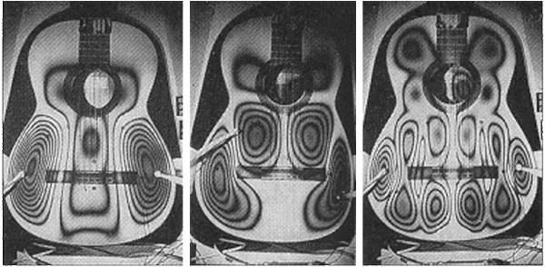

Vibrations of a circular drumhead, and of a real guitar
Gravitational attraction
Another major application of PDEs arose in the theory of gravitational attraction, otherwise known as potential theory. The motivating problem was the gravitational attraction of the Earth, or of any other planet. Newton had modelled planets as perfect spheres, but their true form is closer to that of an ellipsoid. And whereas the gravitational attraction of a sphere is the same as that of a point particle (for distances outside the sphere), the same does not hold for ellipsoids.
Colin Maclaurin made significant headway on these issues in a prizewinning memoir of 1740 and a subsequent book Treatise of Fluxions published in 1742. His first step was to prove that if a fluid of uniform density spins at a uniform speed, under the influence of its own gravity, then the equilibrium shape is an oblate spheroid – an ellipsoid of revolution. He then studied the attractive forces generated by such a spheroid, with limited success. His main result was that if two spheroids have the same foci, and if a particle lies either on the equatorial plane or the axis of revolution, then the force exerted on it by either spheroid is proportional to their masses.
In 1743 Clairaut continued working on this problem in his Théorie de la Figure de la Terre. But the big breakthrough was made by Legendre. He proved a basic property of not just spheroids, but any solid of revolution: if you know its gravitational attraction at every point along its axis, then you can deduce the attraction at any other point. His method was to express the attraction as an integral in spherical polar coordinates. Manipulating this integral, he expressed its value as a superposition of spherical harmonics. These are determined by special functions now called Legendre polynomials. In 1784, he pursued this topic, proving many basic properties of these polynomials.
The fundamental PDE for potential theory is Laplace’s equation, which appears in Laplace’s five-volume Traité de Mécanique Céleste (Treatise on Celestial Mechanics) published from 1799 onwards. It was known to earlier researchers, but Laplace’s treatment was definitive. The equation takes the form

An ellipsoid
![]()
where V(x, y, z) is the potential at a point (x, y, z) in space. Intuitively, it says that the value of the potential at any given point is the average of its values over a tiny sphere surrounding that point. The equation is valid outside the body: inside, it must be modified to what is now known as Poisson’s equation.
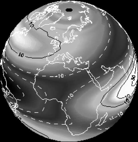
Heat and temperature
Successes with sound and gravitation encouraged mathematicians to turn their attention to other physical phenomena. One of the most significant was heat. At the start of the 19th century the science of heat flow was becoming a highly practical topic, mainly because of the needs of the metalworking industry, but also because of a growing interest in the structure of the Earth’s interior, and in particular the temperature inside the planet. There is no direct way to measure the temperature a thousand miles or more below the Earth’s surface, so the only available methods were indirect, and an understanding of how heat flowed through bodies of various compositions was essential.
In 1807 Joseph Fourier submitted a paper on heat flow to the French Academy of Sciences, but the referees rejected it because it was insufficiently developed. To encourage Fourier to continue the work, the Academy made heat flow the subject of its 1812 grand prize. The prize topic was announced well ahead of time, and by 1811 Fourier had revised his ideas, put them in for the prize, and won. However, his work was widely criticized for its lack of logical rigour and the Academy refused to publish it as a memoir. Fourier, irritated by this lack of appreciation, wrote his own book, Théorie Analytique de la Chaleur (Analytic Theory of Heat), published in 1822. Much of the 1811 paper was included unchanged, but there was extra material too. In 1824 Fourier got even: he was made Secretary of the Academy, and promptly published his 1811 paper as a memoir.
Fourier’s first step was to derive a PDE for heat flow. With various simplifying assumptions – the body must be homogeneous (with the same properties everywhere) and isotropic (no direction within it should behave differently from any other), and so on. He came up with what we now call the heat equation, which describes how the temperature at any point in a three-dimensional body varies with time. The heat equation is very similar in form to Laplace’s equation and the wave equation, but the partial derivative with respect to time is of first order, not second. This tiny change makes a huge difference to the mathematics of the PDE.
‘In 1824 Fourier got even: he was made Secretary of the Academy.’
There were similar equations for bodies in one and two dimensions (rods and sheets) obtained by removing the terms in z (for two dimensions) and then y (for one). Fourier solved the heat equation for a rod (whose length we take to be π), the ends of which are maintained at a fixed temperature, by assuming that at time t = 0 (the initial condition) the temperature at a point x on the rod is of the form
b1 sin x + b2 sin 2x + b3 sin 3x + . . .
(an expression suggested by preliminary calculations) and deduced that the temperature must then be given by a similar but more complicated expression in which each term is multiplied by a suitable exponential function. The analogy with harmonics in the wave equation is striking. But there each mode given by a pure sine function oscillates indefinitely without losing amplitude, whereas here each sinusoidal mode of the temperature distribution decays exponentially with time, and the higher modes decay more rapidly.
The physical reason for the difference is that in the wave equation energy is conserved, so the vibrations cannot die down. But in the heat equation, the temperature diffuses throughout the rod, and is lost at the ends because these are kept cool.
The upshot of Fourier’s work is that whenever we can expand the initial temperature distribution in a Fourier series – a series of sine and cosine functions like the one above – then we can immediately read off how the heat flows through the body as time passes. Fourier considered it obvious that any initial distribution of temperature could be so expressed, and this is where the trouble began, because a few of his contemporaries had been worrying about precisely this issue for some time, in connection with waves, and had convinced themselves that it was much harder than it seemed.
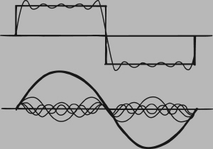
Fourier expansion of a square wave: above, the component sine curves; below, their sum
A typical discontinuous function is the square wave S(x), which takes the values 1 when −π < x ≤ 0 and –1 when 0 < x ≤ π and has period 2π. Applying Fourier’s formula to the square wave we get the series
![]()
The terms add up, as shown in the diagram below.
Although the square wave is discontinuous, every approximation is continuous. However, the wiggles build up as more and more terms are added, making the graph of the Fourier series become increasingly steep near the discontinuities. This is how an infinite series of continuous functions can develop a discontinuity.
Fourier’s argument for the existence of an expansion in sines and cosines was complicated, confused and wildly non-rigorous. He went all round the mathematical houses to derive, eventually, a simple expression for the coefficients b1, b2, b3, etc. Writing f(x) for the initial temperature distribution, his result was
![]()
Euler had already written down this formula in 1777, in the context of the wave equation for sound, and he proved it using the clever observation that distinct modes, sin mπx and sin mπx, are orthogonal, meaning that
![]()
is zero whenever m and n are distinct integers, but non-zero – in fact, equal to π/2 – when m = n. If we assume that f(x) has a Fourier expansion, multiply both sides by sin nx and integrate, then every term except one disappears, and the remaining terms yield Fourier’s formula for bn.
Fluid dynamics
No discussion of the PDEs of mathematical physics would be complete without mentioning fluid dynamics. Indeed, this is an area of enormous practical significance, because these equations describe the flow of water past submarines, of air past aircraft, and even the flow of air past Formula 1 racing cars.
Euler started the subject in 1757 by deriving a PDE for the flow of a fluid of zero viscosity, that is zero ‘stickiness’. This equation remains realistic for some fluids, but it is too simple to be of much practical use. Equations for a viscous fluid were derived by Claude Navier in 1821, and again by Poisson in 1829. They involve various partial derivatives of the fluid velocity. In 1845 George Gabriel Stokes deduced the same equations from more basic physical principles, and they are therefore known as the Navier–Stokes equations.
What differential equations did for them
Kepler’s model of elliptical orbits is not exact. It would be if there were only two bodies in the solar system, but when a third body is present, it changes (perturbs) the elliptical orbit. Because the planets are spaced quite a long way apart, this problem affects the detailed motion, and most orbits remain close to ellipses. However, Jupiter and Saturn behave strangely, sometimes lagging behind where they ought to be and sometimes pulling ahead. This effect is caused by their mutual gravitation, together with that of the Sun.
Newton’s law of gravitation applies to any number of bodies, but the calculations become very difficult when there are three bodies or more. In 1748, 1750 and 1752 the French Academy of Sciences offered prizes for accurate calculations of the movements of Jupiter and Saturn. In 1748 Euler used differential equations to study how Jupiter’s gravity perturbs the orbit of Saturn, and won the prize. He tried again in 1752 but his work contained significant mistakes. However, the underlying ideas later turned out to be useful.
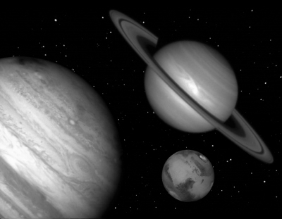
Jupiter and Saturn in a composite picture
1850–1891
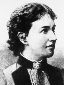
Sofia Kovalevskaya was the daughter of an artillery general and a member of the Russian nobility. It so happened that her nursery walls had been papered with pages from lecture notes on analysis. At the age of 11 she took a close look at her wallpaper and taught herself calculus. She became attracted to mathematics, preferring it to all other areas of study. Her father tried to stop her, but she carried on regardless, reading an algebra book when her parents were sleeping.
In order to travel and obtain an education, she was obliged to marry, but the marriage was never a success. In 1869 she studied mathematics in Heidelberg, but because female students were not permitted, she had to persuade the university to let her attend lectures on an unofficial basis. She showed impressive mathematical talent, and in 1871 she went to Berlin, where she studied under the great analyst Karl Weierstrass. Again, she was not permitted to be an official student, but Weierstrass gave her private lessons.
She carried out original research, and by 1874 Weierstrass said that her work was suitable for a doctorate. She had written three papers, on PDEs, elliptic functions and the rings of Saturn. In the same year Göttingen University awarded her a doctoral degree. The PDE paper was published in 1875.
In 1878 she had a daughter, but returned to mathematics in 1880, working on the refraction of light. In 1883 her husband, from whom she had separated, committed suicide, and she spent more and more time working on her mathematics to assuage her feelings of guilt. She obtained a university position in Stockholm, giving lectures in 1884. In 1889 she became the third female professor ever at a European university, after Maria Agnesi (who never took up her post) and the physicist Laura Bassi. Here she did research on the motion of a rigid body, entered it for a prize offered by the Academy of Sciences in 1886, and won. The jury found the work so brilliant that they increased the prize money. Subsequent work on the same topic was awarded a prize by the Swedish Academy of Sciences, and led to her being elected to the Imperial Academy of Sciences.
Ordinary differential equations
We close this section with two far-reaching contributions to the use of ODEs (ordinary differential equations) in mechanics. In 1788 Lagrange published his Mécanique Analytique (Analytical Mechanics), proudly pointing out that
‘One will not find figures in this work. The methods that I expound require neither constructions, nor geometrical or mechanical arguments, but only algebraic operations, subject to a regular and uniform course.’
At that period, the pitfalls of pictorial arguments had become apparent, and Lagrange was determined to avoid them. Pictures are now back in vogue, though supported by solid logic, but Lagrange’s insistence on a formal treatment of mechanics inspired a new unification of the subject, in terms of generalized coordinates. Any system can be described using many different variables. For a pendulum, for instance, the usual coordinate is the angle at which the pendulum is hanging, but the horizontal distance between the bob and the vertical would do equally well.
The equations of motion look very different in different coordinate systems, and Lagrange felt this was inelegant. He found a way to rewrite the equations of motion in a form that looks the same in every coordinate system. The first innovation is to pair off the coordinates: to every position coordinate q (such as the angle of the pendulum) there is associated the corresponding velocity coordinate, ![]() (the rate of angular motion of the pendulum). If there are k position coordinates, there are also k velocity coordinates. Instead of a second-order differential equation in the positions, Lagrange derived a first-order differential equation in the positions and the velocities. He formulated this in terms of a quantity now called the Lagrangian.
(the rate of angular motion of the pendulum). If there are k position coordinates, there are also k velocity coordinates. Instead of a second-order differential equation in the positions, Lagrange derived a first-order differential equation in the positions and the velocities. He formulated this in terms of a quantity now called the Lagrangian.
Hamilton improved Lagrange’s idea, making it even more elegant. Physically, he used momentum instead of velocity to define the extra coordinates. Mathematically, he defined a quantity now called the Hamiltonian, which can be interpreted – for many systems – as energy. Theoretical work in mechanics generally uses the Hamiltonian formalism, which has been extended to quantum mechanics as well.
What differential equations do for us
There is a direct link between the wave equation and radio and television.
Around 1830 Michael Faraday carried out experiments on electricity and magnetism, investigating the creation of a magnetic field by an electric current, and an electric field by a moving magnet. Today’s dynamos and electric motors are direct descendants from his apparatus. In 1864 James Clerk Maxwell reformulated Faraday’s theories as mathematical equations for electromagnetism: Maxwell’s equations. These are PDEs involving the magnetic and electric fields.
A simple deduction from Maxwell’s equations leads to the wave equation. This calculation shows that electricity and magnetism can travel together like a wave, with the speed of light. What travels at the speed of light? Light. So light is an electromagnetic wave. The equation placed no limitations on the frequency of the wave, and light waves occupy a relatively small range of frequencies, so physicists deduced that there ought to be electromagnetic waves with other frequencies. Heinrich Hertz demonstrated the physical existence of such waves, and Guglielmo Marconi turned them into a practical device: radio. The technology snowballed. Television and radar also rely on electromagnetic waves. So do GPS satellite navigation, mobile phones and wireless computer communications.
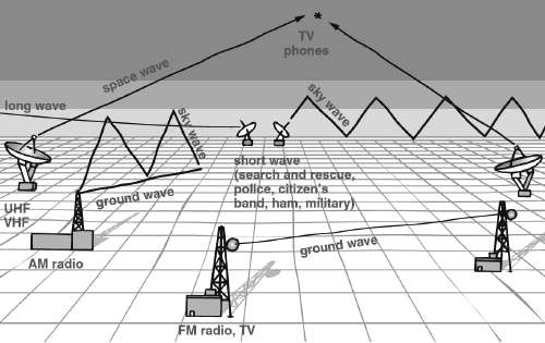
Radio waves
Physics goes mathematical
Newton’s Principia was impressive, with its revelation of deep mathematical laws underlying natural phenomena. But what happened next was even more impressive. Mathematicians tackled the entire panoply of physics – sound, light, heat, fluid flow, gravitation, electricity, magnetism. In every case, they came up with differential equations that described the physics, often very accurately.
The long-term implications have been remarkable. Many of the most important technological advances, such as radio, television and commercial jet aircraft depend, in numerous ways, on the mathematics of differential equations. The topic is still the subject of intense research activity, with new applications emerging almost daily. It is fair to say that Newton’s invention of differential equations, fleshed out by his successors in the 18th and 19th centuries, is in many ways responsible for the society in which we now live. This only goes to show what is lurking just behind the scenes, if you care to look.
‘. . .radio, television and commercial jet aircraft depend on the mathematics of differential equations.’