18

How Likely is That?

The rational approach to chance

The growth of mathematics in the 20th and early 21st centuries has been explosive. More new mathematics has been discovered in the last 100 years than in the whole of previous human history. Even to sketch these discoveries would take thousands of pages, so we are forced to look at a few samples from the enormous amount of material that is available.

An especially novel branch of mathematics is the theory of probability, which studies the chances associated with random events. It is the mathematics of uncertainty. Earlier ages scratched the surface, with combinatorial calculations of odds in gambling games and methods for improving the accuracy of astronomical observations despite observational errors, but only in the early 20th century did probability theory emerge as a subject in its own right.

Probability and statistics

Nowadays, probability theory is a major area of mathematics, and its applied wing, statistics, has a significant effect on our everyday lives – possibly more significant than any other single major branch of mathematics. Statistics is one of the main analytic techniques of the medical profession. No drug comes to market, and no treatment is permitted in a hospital, until clinical trials have ensured that it is sufficiently safe, and that it is effective. Safety here is a relative concept: treatments may be used on patients suffering from an otherwise fatal disease when the chance of success would be far too small to use them in less serious cases.

Probability theory may also be the most widely misunderstood, and abused, area of mathematics. But used properly and intelligently, it is a major contributor to human welfare.

Games of chance

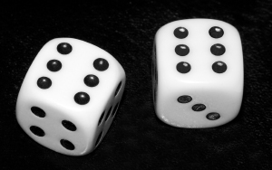
A few probabilistic questions go back to antiquity. In the Middle Ages, we find discussions of the chances of throwing various numbers with two dice. To see how this works, let’s start with one die. Assuming that the die is fair – which turns out to be a difficult concept to pin down – each of the six numbers 1, 2, 3, 4, 5 and 6 should be thrown equally often, in the long run. In the short run, equality is impossible: the first throw must result in just one of those numbers, for instance. In fact, after six throws it is actually rather unlikely to have thrown each number exactly once. But in a long series of throws, or trials, we expect each number to turn up roughly one time in six; that is, with probability ¹/₆. If this didn’t happen, the die would in all likelihood be unfair or biased.

An event of probability 1 is certain, and one of probability 0 is impossible. All probabilities lie between 0 and 1, and the probability of an event represents the proportion of trials in which the event concerned happens.

Back to that medieval question. Suppose we throw two dice simultaneously (as in numerous games from craps to Monopoly^™). What is the probability that their sum is 5? The upshot of numerous arguments, and some experiments, is that the answer is ¹/₉. Why? Suppose we distinguish the two dice, colouring one blue and the other red. Each die can independently yield six distinct numbers, making a total of 36 possible pairs of numbers, all equally likely. The combinations (blue + red) that yield 5 are 1 + 4, 2 + 3, 3 + 2, 4 + 1; these are distinct cases because the blue die produces distinct results in each case, and so does the red one. So in the long run we expect to find a sum of 5 on four occasions out of 36, a probability of ⁴/₃₆ = ¹/₉.

Another ancient problem, with a clear practical application, is how to divide the stakes in a game of chance if the game is interrupted for some reason. The Renaissance algebraists Pacioli, Cardano, and Tartaglia all wrote on this question. Later, the Chevalier de Meré asked Pascal the same question, and Pascal and Fermat wrote each other several letters on the topic.

From this early work emerged an implicit understanding of what probabilities are and how to calculate them. But it was all very ill-defined and fuzzy.

Combinations

A working definition of the probability of some event is the proportion of occasions on which it will happen. If we roll a die, and the six faces are equally likely, then the probability of any particular face showing is ¹/₆. Much early work on probability relied on calculating how many ways some event would occur, and dividing that by the total number of possibilities.

A basic problem here is that of combinations. Given, say, a pack of six cards, how many different subsets of four cards are there? One method is to list these subsets: if the cards are 1 − 6, then they are

1234	1235	1236	1245	1246
1256	1345	1346	1356	1456
2345	2346	2356	2456	3456

so there are 15 of them. But this method is too cumbersome for larger numbers of cards, and something more systematic is needed.

Imagine choosing the members of the subset, one at a time. We can choose the first in six ways, the second in only five (since one has been eliminated), the third in four ways, the fourth in three ways. The total number of choices, in this order, is 6 × 5 × 4 × 3 = 360. However, every subset is counted 24 times – as well as 1234 we find 1243, 2134, and so on, and there are 24 (4 × 3 × 2) ways to rearrange four objects. So the correct answer is 360/24, which equals 15. This argument shows that the number of ways to choose m objects from a total of n objects is

These expressions are called binomial coefficients, because they also arise in algebra. If we arrange them in a table, so that the nth row contains the binomial coefficients

then the result looks like this:

In the sixth row we see the numbers 1, 6, 15, 20, 15, 6, 1. Compare with the formula (x + 1)⁶ = x⁶ + 6x⁵ + 15x⁴ + 20x³ + 15x² + 6x + 1 and we see the same numbers arising as the coefficients. This is not a coincidence.

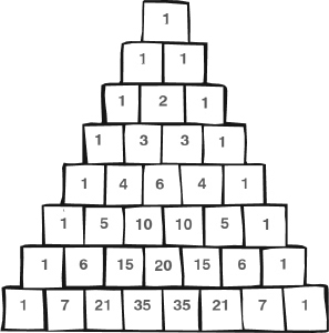
Pascal’s triangle

The triangle of numbers is called Pascal’s triangle because it was discussed by Pascal in 1655. However, it was known much earlier; it goes back to about 950 in a commentary on an ancient Indian book called the Chandas Shastra. It was also known to the Persian mathematicians Al-Karaji and Omar Khayyám, and is known as the Khayyám triangle in modern Iran.

Probability theory

Binomial coefficients were used to good effect in the first book on probability: the Ars Conjectandi (Art of Conjecturing) written by Jacob Bernoulli in 1713. The curious title is explained in the book:

‘We define the art of conjecture, or stochastic art, as the art of evaluating as exactly as possible the probabilities of things, so that in our judgments and actions we can always base ourselves on what has been found to be the best, the most appropriate, the most certain, the best advised; this is the only object of the wisdom of the philosopher and the prudence of the statesman.’

So a more informative translation might be The Art of Guesswork.

Bernoulli took it for granted that more and more trials lead to better and better estimates of probability.

‘Suppose that without your knowledge there are concealed in an urn 3000 white pebbles and 2000 black pebbles, and in trying to determine the numbers of these pebbles you take out one pebble after another (each time replacing the pebble. . .) and that you observe how often a white and how often a black pebble is drawn. . . Can you do this so often that it becomes ten times, one hundred times, one thousand times, etc, more probable. . . that the numbers of whites and blacks chosen are in the same 3:2 ratio as the pebbles in the urn, rather than a different ratio?’

Here Bernoulli asked a fundamental question, and also invented a standard illustrative example, balls in urns. He clearly believed that a ratio of 3:2 was the sensible outcome, but he also recognized that actual experiments would only approximate this ratio. But he believed that with enough trials, this approximation should become better and better.

There is a difficulty here, and it stymied the whole subject for a long time. In such an experiment, it is certainly possible that by pure chance every pebble removed could be white. So there is no hard and fast guarantee that the ratio must always tend to 3:2. The best we can say is that with very high probability, the numbers should approach that ratio. But now there is a danger of circular logic: we use ratios observed in trials to infer probabilities, but we also use probabilities to carry out that inference. How can we observe that the probability of all pebbles being white is very small? If we do that by lots of trials, we have to face the possibility that the result there is misleading, for the same reason; and the only way out seems to be even more trials to show that this event is itself highly unlikely. We are caught in what looks horribly like an infinite regress.

What probability did for them

In 1710 John Arbuthnot presented a paper to the Royal Society in which he used probability theory as evidence for the existence of God. He analysed the annual number christenings for male and female children for the period 1629–1710, and found that there are slightly more boys than girls. Moreover, the figure was pretty much the same in every year. This fact was already well known, but Arbuthnot proceeded to calculate the probability of the proportion being constant. His result was very small, 2^-82. He then pointed out that if the same effect occurs in all countries, and at all times throughout history, then the chances are even smaller, and concluded that divine providence, not chance, must be responsible.

On the other hand, in 1872 Francis Galton used probabilities to estimate the efficacy of prayer by noting that prayers were said every day, by huge numbers of people, for the health of the royal family. He collected data and tabulated the ‘mean age attained by males of various classes who had survived their 30th year, from 1758 to 1843,’ adding that ‘deaths by accident are excluded.’ These classes were eminent men, royalty, clergy, lawyers, doctors, aristocrats, gentry, tradesmen, naval officers, literature and science, army officers, and practitioners of the fine arts. He found that ‘The sovereigns are literally the shortest lived of all who have the advantage of affluence. The prayer has therefore no efficacy, unless the very questionable hypothesis be raised, that the conditions of royal life may naturally be yet more fatal, and that their influence is partly, though incompletely, neutralized by the effects of public prayers.’

Fortunately, the early investigators of probability theory did not allow this logical difficulty to stop them. As with calculus, they knew what they wanted to do, and how to do it. Philosophical justification was less interesting than working out the answers.

Bernoulli’s book contained a wealth of important ideas and results. One, the Law of Large Numbers, sorts out in exactly what sense long-term ratios of observations in trials correspond to probabilities. Basically, he proves that the probability that the ratio does not become very close to the correct probability tends to zero as the number of trials increases without limit.

Another basic theorem can be viewed in terms of repeatedly tossing a biased coin, with a probability p of giving heads, and q = 1 − p of giving tails. If the coin is tossed twice, what is the probability of exactly 2, 1 or 0 heads? Bernoulli’s answer was p², 2pq and q². These are the terms arising from the expansion of (p + q)² as p² + 2pq + q². Similarly if the coin is tossed three times, the probabilities of 3, 2, 1 or 0 heads are the successive terms in (p + q)³ = p³ + 3p²q + 3q²p + q³.

More generally, if the coin is tossed n times, the probability of exactly m heads is equal to

the corresponding term in the expansion of (p + q)ⁿ.

Between 1730 and 1738 Abraham De Moivre extended Bernoulli’s work on biased coins. When m and n are large, it is difficult to work out the binomial coefficient exactly, and De Moivre derived an approximate formula, relating Bernoulli’s binomial distribution to what we now call the error function or normal distribution

De Moivre was arguably the first person to make this connection explicit. It was to prove fundamental to the development of both probability theory and statistics.

Defining probability

A major conceptual problem in probability theory was to define probability. Even simple examples – where everyone knew the answer – presented logical difficulties. If we toss a coin, then in the long run, we expect equal numbers of heads and tails, and the probability of each is ½. More precisely, this is the probability provided the coin is fair. A biased coin might always turn up heads. But what does ‘fair’ mean? Presumably, that heads and tails are equally likely. But the phrase ‘equally likely’ refers to probabilities. The logic seems circular. In order to define probability, we need to know what probability is.

The way out of this impasse is one that goes back to Euclid, and was brought to perfection by the algebraists of the late 19th and early 20th centuries. Axiomatize. Stop worrying about what probabilities are. Write down the properties that you want probabilities to possess, and consider those to be axioms. Deduce everything else from them.

The question was: what are the right axioms? When probabilities refer to finite sets of events, this question has a relatively easy answer. But applications of probability theory often involved choices from potentially infinite sets of possibilities. If you measure the angle between two stars, say, then in principle that can be any real number between 0° and 180°. There are infinitely many real numbers. If you throw a dart at a board, in such a way that in the long run it has the same chance of hitting any point on the board, then the probability of hitting a given region should be the area of that region, divided by the total area of the dartboard. But there are infinitely many points on a dartboard, and infinitely many regions.

These difficulties caused all sorts of problems, and all sorts of paradoxes. They were finally resolved by a new idea from analysis, the concept of a measure.

Analysts working on the theory of integration found it necessary to go beyond Newton, and define increasingly sophisticated notions of what constitutes an integrable function, and what its integral is. After a series of attempts by various mathematicians, Henri Lebesgue managed to define a very general type of integral, now called the Lebesgue integral, with many pleasant and useful analytic properties.

The key to his definition was Lebesgue measure, which is a way to assign a concept of length to very complicated subsets of the real line. Suppose that the set consists of non-overlapping intervals of lengths 1, ½, ¼, ⅛ and so on. These numbers form a convergent series, with sum 2. So Lebesgue insisted that this set has measure 2. Lebesgue’s concept has a new feature: it is countably additive. If you put together an infinite collection of non-overlapping sets, and if this collection is countable in Cantor’s sense, with cardinal א₀, then the measure of the whole set is the sum of the infinite series formed by the measures of the individual sets.

In many ways the idea of a measure was more important than the integral to which it led. In particular, probability is a measure. This property was made explicit in the 1930s by Andrei Kolmogorov, who laid down axioms for probabilities. More precisely, he defined a probability space. This comprises a set X, a collection B of subsets of X called events and a measure m on B. The axioms state that m is a measure, and that m(X) = 1 (that is, the probability that something happens is always 1.) The collection B is also required to have some set-theoretic properties that allow it to support a measure.

For a die, the set X consists of the numbers 1–6, and the set B contains every subset of X. The measure of any set Y in B is the number of members of Y, divided by 6. This measure is consistent with the intuitive idea that each face of the die has probability ¹/₆ of turning up. But the use of a measure requires us to consider not just faces, but sets of faces. The probability associated with some such set Y is the probability that some face in Y will turn up. Intuitively, this is the size of Y divided by 6.

With this simple idea, Kolmogorov resolved several centuries of often heated controversy, and created a rigorous theory of probability.

Statistical data

The applied arm of probability theory is statistics, which uses probabilities to analyse real world data. It arose from 18th century astronomy, when observational errors had to be taken into account. Empirically and theoretically, such errors are distributed according to the error function or normal distribution, often called the bell curve because of its shape. Here the error is measured horizontally, with zero error in the middle, and the height of the curve represents the probability of an error of given size. Small errors are fairly likely, whereas large ones are very improbable.

The bell curve

In 1835 Adolphe Quetelet advocated using the bell curve to model social data – births, deaths, divorces, crime and suicide. He discovered that although such events are unpredictable for individuals, they have statistical patterns when observed for an entire population. He personified this idea in terms of the ‘average man’, a fictitious individual who was average in every respect. To Quetelet, the average man was not just a mathematical concept: it was the goal of social justice.

From about 1880 the social sciences began to make extensive use of statistical ideas, especially the bell curve, as a substitute for experiments. In 1865 Francis Galton made a study of human heredity. How does the height of a child relate to that of its parents? What about weight, or intellectual ability? He adopted Quetelet’s bell curve, but saw it as a method for separating distinct populations, not as a moral imperative. If certain data showed two peaks, rather than the single peak of the bell curve, then that population must be composed of two distinct sub-populations, each following its own bell curve. By 1877 Galton’s investigations were leading him to invent regression analysis, a way of relating one data set to another to find the most probable relationship.

Quetelet’s graph of how many people have a given height: height runs horizontally, the number of people vertically

Another key figure was Ysidor Edgeworth. Edgeworth lacked Galton’s vision, but he was a far better technician, and he put Galton’s ideas on a sound mathematical basis. A third was Karl Pearson, who developed the mathematics considerably. But Pearson’s most effective role was that of salesman: he convinced the outside world that statistics was a useful subject.

What probability does for us

A very important use of probability theory occurs in medical trials of new drugs. These trials collect data on the effects of the drugs – do they seem to cure some disorder, or do they have unwanted adverse effects? Whatever the figures seem to indicate, the big question here is whether the data are statistically significant. That is, do the data result from a genuine effect of the drug, or are they the result of pure chance? This problem is solved using statistical methods known as hypothesis testing. These methods compare the data with a statistical model, and estimate the probability of the results arising by chance. If, say, that probability is less than 0.01, then with probability 0.99 the data are not due to chance. That is, the effect is significant at the 99% level. Such methods make it possible to determine, with considerable confidence, which treatments are effective, or which produce adverse effects and should not be used.

Newton and his successors demonstrated that mathematics can be a very effective way to understand the regularities of nature. The invention of probability theory, and its applied wing, statistics, made the same point about the irregularities of nature. Remarkably, there are numerical patterns in chance events. But these patterns show up only in statistical quantities such as long-term trends and averages. They make predictions, but these are about the likelihood of some event happening or not happening. They do not predict when it will happen. Despite that, probability is now one of the most widely used mathematical techniques, employed in science and medicine to ensure that any deductions made from observations are significant, rather than apparent patterns resulting from chance associations.