Regression trees

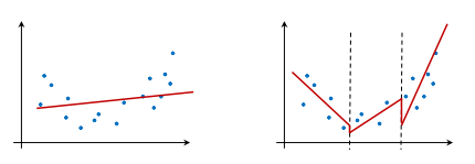
Another approach is to construct a set of regression models, each on its own part of the data. The following diagram shows the main difference between a regression model and a regression tree. A regression model constructs a single model that best fits all of the data. A regression tree, on the other hand, constructs a set of regression models, each modeling a part of the data, as shown on the right-hand side. Compared to the regression model, the regression tree can better fit the data, but the function is a piece-wise linear plot, with jumps between modeled regions, as seen in the following diagram:

A regression tree in Weka is implemented within the M5 class. The model construction follows the same paradigm: initialize the model, pass the parameters and data, and invoke the buildClassifier(Instances) method, as follows:

import weka.classifiers.trees.M5P; 
... 
M5P md5 = new M5P(); 
md5.setOptions(new String[]{""}); 
md5.buildClassifier(data);  
System.out.println(md5); 

The induced model is a tree with equations in the leaf nodes, as follows:

    M5 pruned model tree:
    (using smoothed linear models)
    
    X1 <= 0.75 : 
    |   X7 <= 0.175 : 
    |   |   X1 <= 0.65 : LM1 (48/12.841%)
    |   |   X1 >  0.65 : LM2 (96/3.201%)
    |   X7 >  0.175 : 
    |   |   X1 <= 0.65 : LM3 (80/3.652%)
    |   |   X1 >  0.65 : LM4 (160/3.502%)
    X1 >  0.75 : 
    |   X1 <= 0.805 : LM5 (128/13.302%)
    |   X1 >  0.805 : 
    |   |   X7 <= 0.175 : 
    |   |   |   X8 <= 1.5 : LM6 (32/20.992%)
    |   |   |   X8 >  1.5 : 
    |   |   |   |   X1 <= 0.94 : LM7 (48/5.693%)
    |   |   |   |   X1 >  0.94 : LM8 (16/1.119%)
    |   |   X7 >  0.175 : 
    |   |   |   X1 <= 0.84 : 
    |   |   |   |   X7 <= 0.325 : LM9 (20/5.451%)
    |   |   |   |   X7 >  0.325 : LM10 (20/5.632%)
    |   |   |   X1 >  0.84 : 
    |   |   |   |   X7 <= 0.325 : LM11 (60/4.548%)
    |   |   |   |   X7 >  0.325 : 
    |   |   |   |   |   X3 <= 306.25 : LM12 (40/4.504%)
    |   |   |   |   |   X3 >  306.25 : LM13 (20/6.934%)
    
    LM num: 1
    Y1 = 
      72.2602 * X1 
      + 0.0053 * X3 
      + 11.1924 * X7 
      + 0.429 * X8 
      - 36.2224
    
    ...
    
    LM num: 13
    Y1 = 
      5.8829 * X1 
      + 0.0761 * X3 
      + 9.5464 * X7 
      - 0.0805 * X8 
      + 2.1492
    
    Number of Rules : 13
  

The tree has 13 leaves, each corresponding to a linear equation. The preceding output is visualized in the following diagram:

The tree can be read similarly to a classification tree. The most important features are at the top of the tree. The terminal node, the leaf, contains a linear regression model explaining the data that reaches this part of the tree.

An evaluation will provide the following results as output:

    Correlation coefficient                  0.9943
    Mean absolute error                      0.7446
    Root mean squared error                  1.0804
    Relative absolute error                  8.1342 %
    Root relative squared error             10.6995 %
    Total Number of Instances              768