13
Examples for Complex Systems

13.1 Introduction

In the previous chapters, phase equilibria as well as chemical equilibria have been thoroughly discussed. For the development of a process model, it is the usual way to describe the chemical reactions first and then focus on the phase equilibria for the separation process. However, there are some substances where special models have to be developed, as phase equilibria and chemical reactions have a strong influence on each other. Furthermore, components occur that do not exist in the pure form so that pure component properties cannot be assigned in the usual way.

The strategy for the development of a process model mentioned above cannot be applied in these cases. In this chapter, two examples for special process models are presented.

13.2 Formaldehyde Solutions

Formaldehyde is one of the most important basic chemical compounds [1]. Aqueous formaldehyde solutions are used as disinfection and conservation agents. It is an educt for the production of resins from phenol, urea, and melamine. Water‐free formaldehyde is the raw material for polyoxymethylene, a dimensionally stable polymer.

Formaldehyde is a low‐boiling substance with a normal boiling point of approximately 254 K. It is not stable in its pure form, so it usually occurs in aqueous or methanolic solutions. Mixtures of formaldehyde and water or alcohols are not binary solutions in the usual sense, as formaldehyde reacts with both of them to a wide variety of species that are not stable as pure compounds themselves. Therefore, the standard procedure for building up a thermodynamic model by setting up the pure component properties and the binary interaction parameters fails in this case. The formaldehyde–water–methanol system is a good example for a reactive phase equilibrium, where a special model has to be developed. This has been done by the group of Maurer [2–6].

The reaction of formaldehyde with water leads to methylene glycol:

13.1

which does, as mentioned, not exist as a pure substance. Further addition of formaldehyde molecules results in the homologous series of methylene glycols according to the reactions

13.2

Similarly, the reactions with alcohols are

13.3

where the products are called hemiformals, which are again not stable as pure substances. Also, hemiformal chains can be formed according to

13.4

The most important hemiformals are the ones formed by the reaction of formaldehyde with methanol (RCH₃ in reaction 13.3). In the following section, the higher methylene glycols and hemiformals are named MG_i and HF_i, respectively.

These chemical reactions have a significant influence on the physical properties of the solution and on the phase equilibria. The formaldehyde, which would normally be expected preferably in the vapor phase, behaves now like a component with a similar vapor pressure as water and methanol. To create a model, the reactions listed above have to be taken into account, at least to an extent where significant amounts of the higher methylene glycols or hemiformals are formed.

The particular difficulty in the Maurer model is that the species created in these reactions do not exist in pure form. Therefore, their vapor pressures and their binary parameters with other components cannot be determined in the usual way. Moreover, methylene glycols and hemiformals can exist simultaneously only in ternary and higher mixtures of water (W), formaldehyde (FA), and methanol (MeOH).

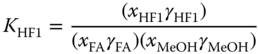
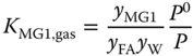
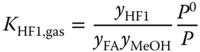
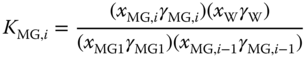
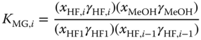
To reduce the number of adjustable parameters, a UNIFAC‐like method (see Section 5.10.3) with special groups for the species occurring in formaldehyde mixtures has been introduced. The groups and their size and surface parameters are given in Table 13.1. For the reactions mentioned above, the mass action laws come into operation. For methylene glycols and hemiformals, the equilibrium constants are given by

13.5

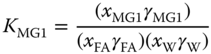
Table 13.1 Main groups of the Maurer model with their volume and surface area parameters [6] .

No.	Main group	R	Q	Group assignment example
1	CH2O	0.9183	0.780	Formaldehyde: 1CH2O
2	H2O	0.9200	1.400	Water: 1H2O
3	HO(CH2O)H	2.6744	2.940	Methylene glycol 1: 1HO(CH2O)H
4	OH	1.0000	1.200	Methylene glycol 2 : 1CH2O, 2OH, 1CH2
5	CH2	0.6744	0.540	Methylene glycol 2: 1CH2O, 2OH, 1CH2
6	CH3O	1.1459	1.088	Hemiformal 1: 1CH3O, 1CH2OH
7	CH3OH	1.4311	1.432	Methanol: 1CH3OH
8	CH2OH	1.2044	1.124	Hemiformal 1: 1CH3O, 1CH2OH

and

13.6

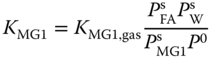
The equilibrium constants for the liquid phase are related to the equilibrium constants for the vapor phase via

13.7

and

13.8

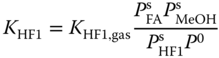
where P⁰ = 101325 Pa and

13.9

13.10

assuming an ideal vapor phase. Similarly, for the higher methylene glycols and hemiformals, the chemical equilibria are described by

13.11

and

13.12

The equilibrium constants, the UNIFAC interaction parameters, and the vapor pressure parameters of the components that do not exist in pure form have to be fitted simultaneously to phase equilibrium data and reaction equilibrium data obtained from spectroscopic measurements for the systems formaldehyde–water and formaldehyde–methanol and the ternary system formaldehyde–water–methanol, for which large amounts of data are available. To keep the significance of the particular parameters, a number of simplifying assumptions are made:

• The vapor pressures of the higher methylene glycols and hemiformals MG_i and HF_i, with i ≥ 2, are set to zero. Therefore, they do not occur in the vapor phase according to the model.
• The reaction constants for the formation of higher methylene glycols with i ≥ 3, and for the formation of higher hemiformals with i ≥ 2, are identical.
• The vapor phase is considered to be ideal.
• Several UNIFAC interaction parameter pairs are set to zero or supposed to be identical.

The final parameter sets used in the Maurer model are given in Tables 13.2–13.4.

Table 13.2 Group interaction parameters a_nm (K) for the UNIFAC approach in the Maurer model [6] .

n/m	1	2	3	4	5	6	7	8
1	—	867.8	189.2	237.7	83.4	0	238.4	238.4
2	−254.5	—	189.2	−229.1	300.0	−219.3	289.6	a28
3	59.2	−191.8	—	−229.1	300.0	−142.4	289.6	289.6
4	28.1	353.5	353.5	—	156.4	112.8	−137.1	−137.1
5	251.5	1318.0	1318.0	986.5	—	447.8	697.2	697.2
6	0	423.8	774.8	1164.8	273.0	—	238.4	238.4
7	−128.6	−181.0	−181.0	249.1	16.5	−128.6	—	0
8	−128.6	a82	−181	249.1	16.5	−128.6	0	—

a₂₈ = 451.64 – 114100 K/T, a₈₂ = −1018.57 + 329900 K/T(parameters are temperature‐dependent).

Table 13.3 Chemical equilibrium constants in the Maurer model [6] : ln K = A + B/(T/K) + C(T/K) + D(T/K)².

	A	B	C	D
KMG1,gas	−16.984	5233.2	—	—
KMG2	0.005019	834.5	—	—
KMGn, n > 2	0.01312	542.1	—	—
KHF1,gas	56.364	0	−0.2509	0.0002758
KHF2	−0.6291	−407.7	–	–
KHFn, n > 2	−0.5018	−526.2	–	–

Table 13.4 Antoine coefficients used in the Maurer model [6] : ln (P^s/kPa) = A + B/[T/K + C].

Component	A	B	C
Formaldehyde	14.4625	−2204.13	−30.00
Water	16.2886	−3816.44	−46.13
Methanol	16.5725	−3626.55	−34.29
Methylene glycol	17.4364	−4762.07	−51.21
Hemiformal	19.5736	−5646.71	0.00

For practical applications, the resulting distribution of the particular methylene glycols and hemiformals is not interesting for the mass balance. It has to be transformed into overall concentrations of formaldehyde, methanol, and water. This is done by applying the formal reactions

13.13

and

13.14

for the final mass balance.

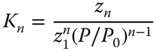
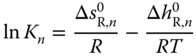
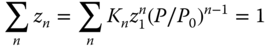
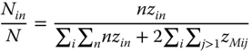
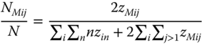
Figures 13.1 and 13.2 give a qualitative overview on the reactive systems formaldehyde–water and formaldehyde–methanol by applying the Maurer model.

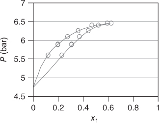
Figure 13.1 The system formaldehyde (1)–water (2) at T = 423 K..

Source: Data from Kuhnert [6]

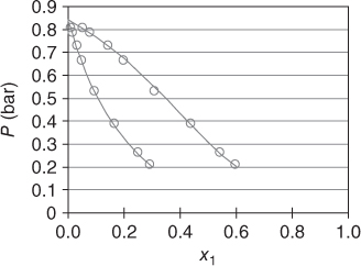
Figure 13.2 The system formaldehyde (1)–methanol (2) at T = 333.1 K..

Source: Data from Kogan and Ogorodnikov [7]

The expected curvature with formaldehyde as a low‐boiling substance is not obtained. Instead, the formaldehyde behaves like a substance with a similar boiling point as water and methanol. For formaldehyde–water, an azeotrope is obtained, which vanishes at high temperatures. The presentations are interrupted at x_FA = 0.6, as for higher concentrations, solid formation is likely to occur. In this area, there are no data points available; thus, the application of the model is not justified. The Maurer model has been successfully applied to several process steps in the polyoxymethylene (POM) production. For this purpose, additional inert components (e.g. trioxane and methylal) have been introduced into the model [3], as well as by‐product reactions like the Cannizzaro reaction

13.15

or the Tischenko reaction [6]

13.16

where formaldehyde is transformed to methyl formate.

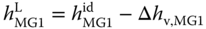
The enthalpies of the methylene glycols and hemiformals can be evaluated by taking into account the enthalpies of the particular formation reactions. For MG₁ and HF₁, it can be written as

13.17

13.18

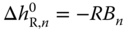
where the enthalpies of reaction are obtained from the van't Hoff equation

13.19

To obtain the liquid enthalpy, the enthalpy of vaporization is subtracted:

13.20

13.21

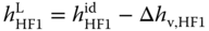
The enthalpies of vaporization can be evaluated with the Clausius–Clapeyron equation (see Section 2.4.4) using the vapor pressure equations given in Table  13.4 . The vapor phase is treated as an ideal gas; this means the vapor phase reality is neglected.

As the vapor pressures of the higher methylene glycols and hemiformals had been set to zero, only their liquid enthalpies are of interest. They can be determined by

13.22

13.23

where the are obtained via the van't Hoff equation analogously to Eq. 13.19. The procedure refers to the enthalpy route A described in Section 6.2. As a derivative of a roughly determined enthalpy of reaction is involved and an ideal gas phase is used, it cannot be expected that the results especially for are very exact. Instead, they must be interpreted as an estimation.

In many cases, the influence of reaction kinetics is significant, especially at low temperatures. On the other hand, the evaluation of the reaction kinetics is difficult because of the number of reactions to be regarded. Moreover, any kinetics must be written with activities and not with concentrations. Otherwise, the results will not be consistent, as the reaction progresses do not move toward the equilibrium state.

In recent works, even a promising application of the slow reaction kinetics has been shown [8]. At low temperatures and low residence times, e.g. in an evaporator, the reaction kinetics are too slow to reach equilibrium. This is advantageous, if the formaldehyde content of the vapor should be as low as possible, which is the case for the enrichment of trioxane by evaporation in the POM process.

The reverse reactions of the MG and HF chains to form MG₁ and molecular formaldehyde are too slow to reach equilibrium; thus, less formaldehyde is evaporated. Different to common absorption processes, the absorption of formaldehyde containing vapors should take place at relatively high temperatures to obtain a sufficient reaction rate in the liquid phase, which is necessary for the absorption.

13.3 Vapor Phase Association

The equations of state described in Section 2.5 take into account that at high pressures the intermolecular forces are no more negligible and the deviations from the ideal gas law become larger. At ambient pressure, the ideal gas law is at least a sufficient approximation to evaluate the PvT behavior.

This is not valid for a certain number of components, i.e. some organic acids and hydrogen fluoride (HF). Table 13.5 shows the compressibility factors of the pure component vapor phase at the normal boiling point, which deviate significantly from the ideal gas law z = Pv/RT = 1.

Table 13.5 Compressibility factors of associating substances at the normal boiling point.

	Normal boiling point (K)	z
Acetic acid	391	0.6
Formic acid	374	0.65
Hydrogen fluoride	293	0.33

According to the association model, it is assumed that these substances form associates in the vapor phase, which themselves behave like an ideal gas. In practical applications, only the occurrence of dimers is taken into account, which is sufficient with respect to the relatively poor data situation. There are two exceptions: for acetic acid, much more experimental data are available, and it makes sense to make the model more flexible and accurate. Just for this purpose, tetramers have been introduced as species, although it has been shown that they actually do not occur to a significant extent [9,10]. As well, for HF quite a lot of data exist. In the vapor phase, a number of different species have been detected. Most often, hexamers occur [11]. The PvT behavior can be successfully described by assuming that there are only monomers and hexamers. The consideration of other species does not result in a better representation.

The character of the association is that of a chemical reaction in the vapor phase. Each reaction

can be described with the law of mass action

13.24

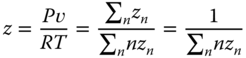
where K is the equilibrium constant (see Chapter 12) and z_n denotes for the true concentration of the associate of the degree n, which means the concentration of the species that consists of n molecules (for n = 1, one gets K₁ = 1). P₀ is an arbitrary reference pressure; in this context, it is chosen as

13.25

The equilibrium constant is related to the Gibbs energy of reaction (see Chapter 12) via

13.26

Therefore, the equilibrium constant can be written as

13.27

Assuming that and are independent of temperature, the correlation function

13.28

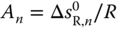with and 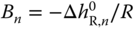is obtained. As the total number of species in the vapor phase is reduced by the association reaction, is always negative, that is, A < 0. Furthermore, the reaction is always exothermic, which means is negative, and therefore B > 0. Values of the association constants for the most important associating substances are given in Table 13.6.

Table 13.6 Association constants for the most important associating substances.

A2	B2/K	A4	B4/K	A6	B6/K
Substance	Formula	Dimerization		Tetramerization		Hexamerization
Formic acid	HCOOH	−29.607	7108	—	—	—	—
Acetic acid	CH3COOH	−29.129	7335	−78.232	17268	—	—
Chloroacetic acid	CH2CICOOH	−43.568	13035	—	—	—	—
Dichloroacetic acid	CHCI2COOH	−38.134	10636	—	—	—	—
Propionic acid	CH3CH2COOH	−29.791	7821	—	—	—	—
Acrylic acid	CH2CHCOOH	−33.989	9384	—	—	—	—
Butyric acid	C3H7COOH	−28.232	7090	—	—	—	—
Benzoic acid	C6H5COOH	−25.467	6012	—	—	—	—
Hydrogen fluoride	HF	—	—	—	—	−119.306	18735

To obtain the true concentrations z_n, the mass balance in the vapor phase has to be evaluated. The sum of the concentrations of the particular species must be 1:

13.29

which results in a nonlinear equation for the monomer concentration z₁. If only dimers are regarded, a quadratic equation

13.30

is obtained, which can be directly solved to

13.31

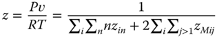
For acetic acid and HF, where tetramers or hexamers are regarded, the equation must be solved numerically, which is, however, pretty easy, as 0 < z₁ < 1. Having calculated z₁, the compressibility factor z can be determined as the ratio between the number of associates and the number of molecules in the vapor phase:

13.32

The specific volume is then obtained via

13.33

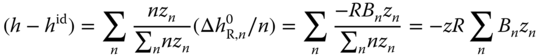
As for all chemical reactions, the enthalpy changes are considerable and cannot be neglected. According to Eqs. 13.27 and 13.28, the enthalpy of reaction is given by

13.34

For each molecule in an association complex of degree n, the contribution to (h − h^id) is equal to . On the other hand, the fraction of molecules being integrated in a complex of degree n is equal to 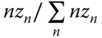. Thus, (h − h^id) can be calculated by

13.35

For comparison with experimental data, it is useful to have an expression for . With

13.36

we obtain

13.37

Due to the complexity of Eq. 13.35, it is recommended to evaluate the differential quotient in Eq. 13.37 numerically.

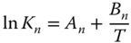
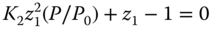
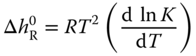
In Figure 13.3, the unusual curvature of the specific heat capacity of gaseous HF as a function of temperature is shown with the pressure as a parameter. For P = 0, it is an almost constant function with . For finite pressures, there is a strong influence of the association reactions, and a peak is formed. For the curve on the left‐hand side, the top of the peak is approximately 40 times larger than . With increasing pressure, the peak becomes less steep, and it is transferred to higher temperatures. The simple association model can reproduce this complicated shape quite well; however, the agreement is not exact.

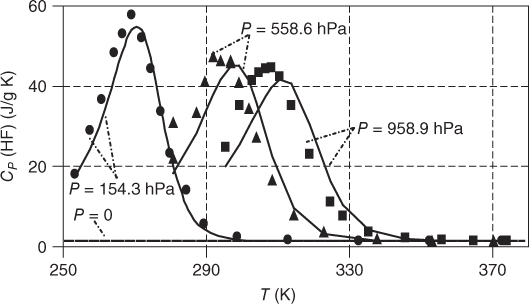
Figure 13.3 Specific heat capacity of gaseous HF as a function of temperature..

Source: Data from Franck and Meyer [12]

The curvature itself is easy to understand: at the boiling point, the vapor consists of hexamers to a large extent. Additional heat supply leads to splitting of hexamers, as it favors the endothermic reaction. The splitting has the character of a chemical reaction; therefore, its energy demand is extremely high. Thus, increases drastically, as the heat is mainly used for the splitting and not for a temperature increase. Finally, with increasing temperature, the number of hexamers to be split decreases; the heat capacity passes a maximum and comes down to the normal value of . The experimental data shown in Figure  13.3 are taken from Franck and Meyer [12] . 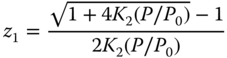For organic acids, the curvature of is similar but less dramatic as it is for HF (Figure 13.4).

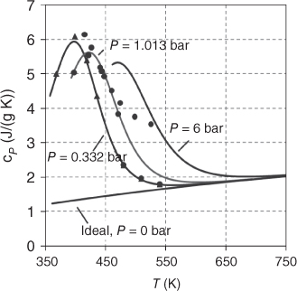
Figure 13.4 of acetic acid vapor as a function of temperature.

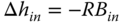
As well, the curvature of the enthalpy of vaporization as a function of temperature is different from the usual ones shown in Figure 3.12. Figure 13.5 shows the plot for HF and acetic acid. Both of them show a maximum value. For HF, the shape is so extraordinary that only the PPDS Eq. (3.62) can yield acceptable correlation results. The Clausius‐Clapeyron equation (3.64) should not be applied for saturation pressures above 1 bar, as the association model does not take into account the physical‐based vapor‐phase nonidealities.

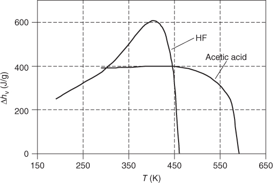
Figure 13.5 Enthalpy of vaporization as a function of temperature for HF and acetic acid.

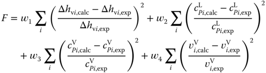
The parameters to describe the equilibrium constants A and B can be fitted to data for vapor density and . Due to the steep shape of the function, relatively small errors cause large contributions to the objective function. Therefore, weighting factors should be introduced to make sure that both types of data are regarded in the evaluation of the objective function. If route A is used for the enthalpy description (Section 6.2 ), it is strongly recommended to integrate data for as well [13]. In this case, the association constants and the coefficients of the correlation of the enthalpy of vaporization are fitted simultaneously to the objective function

13.38

It should be mentioned that there is no chance to estimate association constants. Even qualitative estimations are often dangerous. For example, trichloroacetic acid does not show association behavior [14], although it is more polar than acetic acid, monochloroacetic acid, and dichloroacetic acid.

---

Example 13.1

1. Calculate the specific vapor volume of acetic acid at P = 0.6486 bar and T = 383.15 K.
   Solution

   From Table  13.6 , we get

   

   Eq. 13.29 yields

   

   Starting with an estimated value of z₁ = 0.5, the following iteration is obtained according to the Newton method

   

   With

   

   one gets the following:

   Step	z1,i	f(z1,i)	f′(z1,i)	z1,i + 1
   1	0.5	0.3147	4.3938	0.4284
   2	0.4284	0.0133	3.8156	0.4249
   3	0.4249	−0.00029	3.7884	0.4250
   4	0.4250	0.0001	3.7892	0.4250

   With z₁ = 0.425, Eq. 13.24 yields z₂ = 0.5399 and z₄ = 0.0352. Thus, the compressibility factor is

   

   The specific vapor volume is

   

   According to Barton and Hsu [15], the experimental value is v = 30.0 m³/kmol.

---

Also for pure components, the association model can be applied to mixtures of associating compounds and to mixtures of associating and nonassociating substances. Similarly, the concentrations of the true species can be calculated from material balances. As more than one component occurs, the index system must be revised for K and z. In the following section, the first index denotes for the component, and the second one is the degree of association, for example z₁₂ … true concentration of dimers of component 1.

For mixtures of organic acids, codimers formed by the reaction

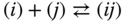
have to be introduced as a new species. The corresponding law of mass action is

13.39

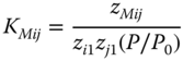
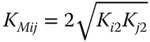
For K_Mij, Prausnitz et al. [16] recommend the relationship

13.40

It has to be distinguished between the true concentrations z_in of the particular species and the apparent concentrations y_i, which represent the stoichiometric mole fractions of the components occurring in the mixture.

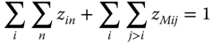
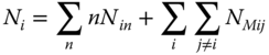
To obtain the true concentrations z_in, a system of equations much more complicated than for pure components must be solved. Again, the true monomer concentrations z_i1 are the key concentrations. After they have been determined, the concentrations of the other species can be derived by the equilibrium conditions Eqs. 13.24 and 13.39. For each component, a true monomer concentration exists, no matter if it associates or not. Therefore, one equation must be available for each component. The first equation of the system is a simple mass balance. The sum of the true concentrations of all species is 1:

13.41

For each component i > 1, an equation can be set up in the following way: the ratio between the numbers of monomers of the particular component and the first component is equal to the ratio of the apparent concentrations:

13.42

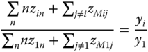
Inserting Eqs. 13.24 and 13.39 , we obtain

13.43

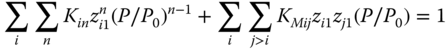
and

13.44

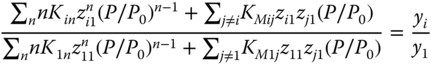
where the values for K_i1 must formally be set to unity.

Thus, a system of nonlinear equations is available to evaluate the true monomer concentrations z_i1, which can be solved with standard methods [17]. The compressibility factor is equal to the ratio between the number of associates and the number of monomers in the associates:

13.45

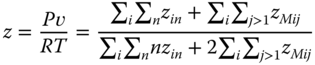
Using Eq. 13.41, it can be written as

13.46

Similarly, the residual part of the vapor enthalpy (h − h^id) can be derived. Using N as the total number of the particular species, it is possible to set up the ratios

13.47

and

13.48

With the help of the van't Hoff equation

13.49

the enthalpies of reaction

13.50

and

13.51

are obtained.

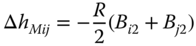
For each molecule in an associate of the degree n (n > 1), the contribution to the enthalpy correction is Δh_in/n or Δh_Mij/2, respectively. Setting Δh_i1 = 0, the enthalpy correction is

13.52

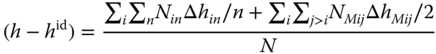
Using Eqs. 13.47 and 13.48, (h − h^id) can be expressed as

13.53

The specific heat capacity can again be calculated according to Eq. 13.37 .

For the calculation of vapor–liquid equilibria (VLE), an analytical expression for the fugacity coefficient is required. It can be derived according to Prausnitz et al. [16] .

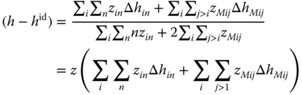
With the material balances for each component

13.54

and the equilibrium conditions for the chemical potentials

13.55

13.56

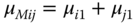
the total differential of the Gibbs energy at constant temperature and pressure is set up in two ways. First, it is formulated without consideration of the true species:

13.57

In the second way, the existence of the particular true species is regarded:

13.58

Substituting the chemical potentials from Eqs. 13.55 and 13.56 in Eq. 13.58, we obtain

13.59

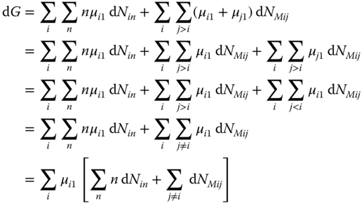
Differentiating Eq. 13.54

13.60

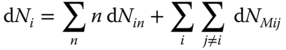
and inserting it into Eq. 13.59, the result is

13.61

The comparison between Eqs. 13.61 and 13.57 yields

13.62

From the stoichiometric point of view, μ_i is the chemical potential of a nonideal gas. Therefore, it can be assigned with a fugacity coefficient:

13.63

From the true component point of view, the evaluation of the chemical potential can be performed by treating the mixture as an ideal gas:

13.64

as the particular species are treated as ideal gases. As for g^pure(T, P⁰) and f⁰ the same conditions are referred to, the fugacity coefficient is simply obtained as

13.65

The association model has been successfully applied in many cases for mixtures containing organic acids or HF. The most important system where it comes into operation is acetic acid/water. Figure 13.6 shows the phase diagram and the representation of the NRTL/association model. For comparison, the fit with NRTL and ideal gas phase is shown as well, demonstrating the considerable quality difference. The same comparison is made for the R22–HF system in Figure 13.7. In this case, only PTx data are available. The fit using the ideal gas model has the same quality as the fit with the association model. However, the vapor concentrations that have not been measured are significantly different.

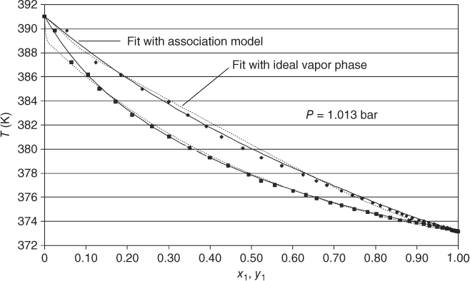
Figure 13.6 Phase diagram for the water (1)–acetic acid (2) system.

Source: Data from Fu et al. [18]. Reproduced with permission from Elsevier.

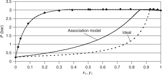
Figure 13.7 Phase diagram for the R22 (1)–HF (2) system..

Source: Data from Wilson et al. [19]

Nevertheless, a model is missing that combines the association model with an equation of state that takes into account the intermolecular forces at high pressures. There are several applications where such a model would be useful [20].

A number of attempts have been made [ 11 21–33]; however, none of them fulfills the particular demands of a process simulator, that is, extension to multicomponent mixtures, proved enthalpy description, and derivation of a fugacity coefficient.

---

Example 13.2

1. Calculate the specific vapor volume of a mixture of 40 mol% formic acid (1) and 60 mol% nitrogen (2) at T = 400 K and P = 1 bar.
   Solution

   According to Table  13.6 , the dimerization constant can be calculated to be

   

   Equations 13.43 and 13.44 yield

   

   From Eq. 13.24 , we get

   

   and

   

   Using Eq. 13.46, we obtain

   

   and

   

---

---

Example 13.3

1. Calculate the fugacity coefficients and for the system water (1)–acetic acid (2) at ϑ = 80 °C with the help of the association model (y₁ = 0.35, P = 35.57 kPa). The required association parameters can be taken from Table  13.6 .
   Solution

   To be able to calculate the fugacity coefficient , first, the equilibrium constants K₂ and K₄ have to be determined at ϑ = 80 °C. Then, the vapor phase mole fraction of the monomeric acetic acid and for water has to be calculated:

   

   Using Eqs. 13.24 , 13.43 , and 13.44 , we get

   

   

   13.66

   and

   13.67

   With P = 35.57 kPa, P₀ = 1 Pa, and the values for K₂₂ and K₂₄ obtained above, we get two equations for z₁₁ and z₂₁:

   

   Eliminating z₁₁ yields

   

   and

   

   This yields z₂₁ = 0.1955 and, subsequently, z₁₁ = 0.4740.

   Using the true mole fractions, the fugacity coefficients can be obtained:

   

   For pure acetic acid, Eq. 13.43 reads

   

   With at ϑ = 80 °C, we obtain

   

   giving

   

---

---

Example 13.4

1. Calculate the activity coefficients for the system water (1)–acetic acid (2) at ϑ = 80 °C for the compositions given in Table 13.7 using Eq. (5.12). The Poynting factor shall be neglected.

   Table 13.7 VLE data for the system water (1)–acetic acid (2) at 80 °C [34,35].

   x1	y1	P (kPa)
   0.0000	0.0000	27.918
   0.0776	0.1480	31.731
   0.1185	0.2040	32.811
   0.1778	0.2810	34.157
   0.2392	0.3500	35.570
   0.3511	0.4590	37.864
   0.4724	0.5800	40.343
   0.6080	0.7100	42.290
   0.6915	0.7820	43.596
   0.7648	0.8400	44.556
   0.8908	0.9240	45.916
   1.0000	1.0000	47.343

   Solution

   This should be shown for the data point at x₁ = 0.2392, since for this data point, the values for the fugacity coefficients have already been calculated in Example 13.3. However, it makes sense to use the experimental vapor pressure of the authors to obtain a more reliable representation (see Appendix F), which causes a small change to . can be set to 1, as pure water does not show association in the vapor phase. The experimental activity coefficients can directly be calculated using Eq. (5.12):

   

   Assuming ideal vapor phase behavior, different activity coefficients are calculated:

   

   

   For all data points, the activity coefficients assuming ideal and real vapor phase behavior are shown in Figure 13.8. It can be recognized that the activity coefficients taking into account nonideal vapor phase behavior show the typical curvature, whereas the ideal calculation results in a very strange curve shape. This is absolutely important for the modeling of the VLE behavior of this system; the dewatering of acetic acid via distillation is quite a difficult task and requires a considerable amount of energy.

   

   Figure 13.8 Activity coefficients calculated for the system water (1)–acetic acid (2) at ϑ = 80 °C taking into account (a) real and (b) ideal vapor phase behavior.

---

Problems

1. 13.1 Calculate the compressibility factor of formic acid vapor at T = 420 K and P = 0.5 bar using the association model. The required dimerization and tetramerization constants can be calculated from the parameters given in Table  13.6 .
2. 13.2 Estimate the heat capacity of acetic acid along the vapor–liquid coexistence curve for both phases using the vapor pressure and ideal gas heat capacity correlations given in Appendix A and the dimerization and tetramerization constants from Table  13.6 .
3. 13.3 Estimate the enthalpy change upon isothermal compression of propionic acid from 0.01 to 1 atm at a temperature of 145 °C using the association model with dimerization constants given in Table  13.6 .
4. 13.4 Estimate the change of the degree of dimerization along the vapor pressure curve for formic acid and propionic acid using the dimerization constants and a simplified vapor pressure equation (log(P^s/1 bar) = A + B/T). Calculate the values of the parameters A and B from the boiling temperatures at P₁ = 0.5 bar and P₂ = 2 bar.

   Boiling points:

   	0.5 bar	2 bar
   Formic acid	78.4 °C	125 °C
   Propionic acid	119.7 °C	164.7 °C

   Dimerization constants can be calculated from the parameters given in Table  13.6 .

5. 13.5 Calculate the saturated vapor pressure and fugacity along the vapor–liquid coexistence curve for benzene, water, and acetic acid between 25 °C and the critical temperature of the components. For the real vapor phase behavior, use the virial equation truncated after the second virial coefficient in the case of water and benzene and the association model in the case of acetic acid. Discuss the results. Which is the temperature range where the results are reliable? Do the calculations lead to under‐ or overprediction of the fugacity outside the reliable temperature range?

   Vapor pressure equation coefficients and second virial coefficient correlations as functions of temperature are given in Appendix A. Dimerization and tetramerization constant parameters are given in Table  13.6 .

6. 13.6 In the case of mixtures of components that do not strongly or differently associate in the vapor phase, the separation factor α_ij can be approximated by . In other cases the ratio of the real gas factors has to be taken into account. Calculate the ratio of the pure component vapor pressures, the activity coefficients (calculated using the UNIQUAC model), and the real gas factors for the system water (1)–acetic acid (2) at 80 °C as function of concentration. Discuss the results.

   Vapor pressure equation constants can be found in Appendix A. Calculate the dimerization and tetramerization constants of acetic acid using the parameters given in Table  13.6 .

   UNIQUAC parameters	Δu12 = 12.0164 cal/mol	Δu21 = 68.3212 cal/mol
   	r1 = 0.9200	q1 = 1.4000
   	r2 = 2.2024	q2 = 2.0720

7. 13.7 Search for experimental heats of vaporization data for acetic acid in the free Dortmund Data Bank Software Package (DDBSP) Explorer Version. Interpret the behavior as function of temperature. Compare the values with those of a nonassociating component of similar molecular weight (acetone).
8. 13.8 In the free DDBSP Explorer Version, search for all data for the system water–acetic acid, and regress these data simultaneously using the three‐suffix Margules equation and binary parameters with quadratic temperature dependence. The three‐suffix Margules g^E model is very seldom used today but is the only simultaneous regression model available in the free DDBSP Explorer Version. In the x–y diagram, the equilibrium curves are nearly parallel to the diagonal line at mole fractions of water greater than 0.7. What is the reason for this strange behavior?
9. 13.9 Calculate the fugacity coefficients of both components in the system acetic acid (1)–water (2) at T = 393.15 K and P = 1 bar for a mole fraction y₁ = 0.5. Use the association model and the corresponding constants from Table  13.6 .

References

1. 1 Walker, J.F. (1964). Formaldehyde. New York: Reinhold Publishing Corporation.
2. 2 Maurer, G. (1986). AlChE J. 32 (6): 932–948.
3. 3 Albert, M., Garcia, B.C., Kuhnert, C. et al. (2000). AlChE J. 46 (8): 1676–1687.
4. 4 Hasse, H. (1990). Dampf‐Flüssigkeits‐Gleichgewichte, Enthalpien und Reaktionskinetik in formaldehydhaltigen Mischungen. PhD thesis. University of Kaiserslautern, Germany.
5. 5 Albert, M. (1999). Thermodynamische Eigenschaften formaldehydhaltiger Mischungen. PhD thesis. University of Kaiserslautern, Germany.
6. 6 Kuhnert, C. (2004). Dampf‐Flüssigkeits‐Gleichgewichte in mehrkomponentigen formaldehydhaltigen Systemen. PhD thesis. University of Kaiserslautern, Germany.
7. 7 Kogan, L.V. and Ogorodnikov, S.K. (1980). Zh. Prikl. Khim. 53 (1): 115–119.
8. 8 Schilling, K., Sohn, M., Ströfer, E., and Hasse, H. (2003). Chem. Ing. Tech. 75 (3): 240–244.
9. 9 Ritter, H.L. and Simons, J.H. (1945). J. Am. Chem. Soc. 67: 757–762.
10. 10 Büttner, R. and Maurer, G. (1983). Ber. Bunsen Ges. Phys. Chem. 87: 877–882.
11. 11 Anderko, A. and Prausnitz, J.M. (1994). Fluid Phase Equilib. 95: 59–71.
12. 12 Franck, E.U. and Meyer, F. (1959). Z. Elektrochem. 63 (5): 571–582.
13. 13 Kleiber, M. (2003). Ind. Eng. Chem. Res. 42: 2007–2014.
14. 14 Landee, F.A. and Johns, I.B. (1941). J. Am. Chem. Soc. 63: 2891–2895.
15. 15 Barton, J.R. and Hsu, C.C. (1969). J. Chem. Eng. Data 14 (2): 184–187.
16. 16 Prausnitz, J.M., Lichtenthaler, R.N., and Azevedo, E.G. (1986). Molecular Thermodynamics of Fluid Phase Equilibria. Prentice‐Hall.
17. 17 Engeln‐Müllges, G. and Reutter, F. (1988). Formelsammlung zur Numerischen Mathematik mit Standard‐FORTRAN 77 Programmen, 6e. Mannheim, Wien, Zürich: BI‐Wissenschaftsverlag.
18. 18 Fu, H., Cheng, G., Han, S. et al. (1986). J. Chem. Eng. (China) 14 (6): 56–61.
19. 19 Wilson, L.C., Wilding, W.V., and Wilson, G.M. (1989). AlChE Symp. Ser. 85 (271): 51.
20. 20 Chem Systems Inc. (1997). Vinyl Acetate. Chem. Systems Rep. 96/97‐5.
21. 21 Anderko, A. (1989). Fluid Phase Equilib. 45: 39–67.
22. 22 Anderko, A. (1989). Chem. Eng. Sci. 44 (3): 713–725.
23. 23 Anderko, A. (1992). Fluid Phase Equilib. 75: 89–103.
24. 24 Derawi, S.O., Zeuthen, J., Michelsen, M.L. et al. (2004). Fluid Phase Equilib. 225: 107–113.
25. 25 Kontogeorgis, G.M., Voutsas, E.C., Yakoumis, I.V., and Tassios, D.P. (1996). Ind. Eng. Chem. Res. 35: 4310–4318.
26. 26 Visco, D.P., Kofke, D.A., and Singh, R.R. (1997). AlChE J. 43 (9): 2381–2384.
27. 27 Chai Kao, C.‐P., Paulaitis, M.E., Sweany, G.A., and Yokozeki, M. (1995). Fluid Phase Equilib. 108: 27–46.
28. 28 Huang, S.H. and Radosz, M. (1990). Ind. Eng. Chem. Res. 29: 2284–2294.
29. 29 Chapman, W.G., Gubbins, K.E., Jackson, G., and Radosz, M. (1990). Ind. Eng. Chem. Res. 29: 1709–1721.
30. 30 Fu, Y.‐H. and Sandler, S.I. (1995). Ind. Eng. Chem. Res. 34: 1897–1909.
31. 31 Gmehling, J., Liu, D.D., and Prausnitz, J.M. (1979). Chem. Eng. Sci. 34: 951–958.
32. 32 Grenzheuser, P. and Gmehling, J. (1986). Fluid Phase Equilib. 25: 1–29.
33. 33 Pang, J. and Peng, D.‐Y. (2006). Fluid Phase Equilib. 241: 31–40.
34. 34 Dortmund Data Bank. Welcome to DDBST GmbH. www.ddbst.com (accessed 16 August 2018).
35. 35 Lazeeva, M.S. and Markuzin, N.P. (1973). J. Appl. Chem. USSR 46 (2): 373–376.