Numerical Evaluation of the Dynamic Response of SDOF Systems
In Section 5.4, Duhamel integral expressions were obtained for the response of undamped and underdamped linear SDOF systems subject to arbitrary excitation. For simple forms of excitation, these expressions can be evaluated in closed form. For more complex excitation, a numerical solution is required. Numerical approximation methods used for simulation of structural dynamics transient response problems fall into two broad categories: integration methods for first- and second-order ordinary differential equations. The two different categories of algorithms have become popular for quite different reasons. The second-order integration methods exploit the structure of the ordinary differential equations so common in structural dynamics. For the most part, the goal of this class of methods is efficiency and accuracy in the numerical integration of the second-order ordinary differential equations of motion. Variants of the second-order methods have been derived for some types of nonlinear ordinary differential equations and are discussed in Section 6.3.2. On the other hand, the first-order methods are typically derived assuming a priori that the underlying equations are nonlinear. They are readily able to accommodate structural dynamics models with nonlinearities. In addition, the first-order forms of the governing equations are more amenable to the study of applications in control theory. Over the past few decades, modern structural dynamics has become closely related to many topics studied in control theory.
Upon completion of this chapter you should be able to:
- Use, and in some cases derive, a number of popular second-order integration methods for applications in structural dynamics. These methods should include:
- Approximation of the excitation via piecewise-constant interpolation
- Approximation of the excitation via piecewise-linear interpolation
- The Average Acceleration Method
- Use, and in some cases derive, a number of first-order integration methods for applications in structural dynamics. These methods should include:
- Direct Taylor Series Methods
- Runge–Kutta Methods
- Multistep Methods
Finally, it is important to note that the collection of techniques summarized above represent only a sample of the useful and viable integration methods for applications in structural dynamics. These methods are, however, representatives of classes of methods that are frequently encountered. This chapter, along with the additional techniques discussed in Chapter 16, should provide an excellent foundation on which the reader can build a more specialized study.
6.1 INTEGRATION OF SECOND-ORDER ORDINARY DIFFERENTIAL EQUATIONS
In this section a number of numerical integration methods are discussed that exploit the structure of the prototypical linear ordinary differential equation
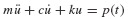
that arises so frequently in structural dynamics. As will be shown in this chapter and in Chapter 16, the algorithms described in this section can be applied to a host of practical problems in structural dynamics.
6.1.1 Numerical Solution Based on Interpolation of the Excitation Function
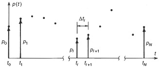
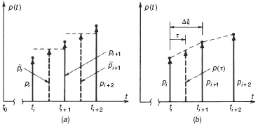
In many practical structural dynamics problems the excitation function, p(t), is not known in the form of an analytical expression, but rather, is given by a set of discrete values pi ≡ p(ti) for i = 0 to N. These may be presented in “tabular form” as a computer file or presented graphically as in Fig. 6.1. The time interval

is frequently taken to be a constant, Δt. One approach to obtaining the response to this excitation is to use numerical quadrature formulas (e.g., the trapezoidal rule or Simpson's one-third rule) to evaluate the integrals appearing in the Duhamel integral expressions of Eqs. 5.36 and 5.37. [6.1] This involves interpolation of the integrands appearing in the Duhamel integrals.
Figure 6.1 Excitation specified at discrete times.
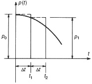
A more direct and efficient procedure involves interpolation of the excitation function p(t) and exact solution of the resulting linear response problem using results from Chapter 5. Figure 6.2 shows piecewise-constant and piecewise-linear interpolation of excitation functions. For piecewise-constant interpolation, the value of the force in the interval ti to ti+1 is  which could be taken to be the value pi at the beginning of the interval, the value pi+1 at the end of the interval, or the average value
 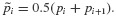 For piecewise-linear interpolation the interpolated force is given by
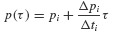
where

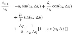
Consider the response of an undamped system. For piecewise-constant interpolation the forced response can be obtained from Eq. 5.8 and the response due to nonzero initial conditions from Eq. 3.17. Thus,
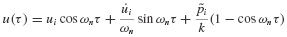
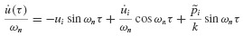
Evaluating these expressions at time ti+1 (i.e., at τ = Δti),we get


Equations 6.5 are the recurrence formulas for evaluating the dynamic state  at time ti+1 given the state
  at time ti.
Figure 6.2 (a) Piecewise-constant and (b) piecewise-linear interpolation of excitation functions.
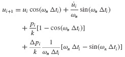
In contrast to piecewise-constant interpolation of the excitation, piecewise-linear interpolation permits a closer approximation. Equation 6.2 can be used to derive recurrence formulas based on piecewise-linear interpolation of the excitation. For an undamped system, we get
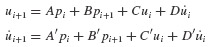
Recurrence formulas such as Eqs. 6.5 and 6.6 may be expressed conveniently in the following form:
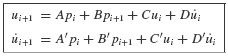
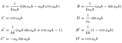
Table 6.1 gives expressions for the coefficients A through D' for the linear force interpolation for the underdamped case (ζ < 1). Coefficients can also be derived for critically damped and overdamped cases.
Table 6.1 Coefficents for Recurrence Formulas for Underdamped SDOF Systems
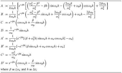
If the time step Δti is constant, the coefficients A through D' need be calculated only once, which greatly speeds the computations. Since the recurrence formulas in Table 6.1 are based on exact integration of the equation of motion for the various force interpolations, the only restriction on the size of the time step Δti is that it permit a close approximation to the excitation and that it provide output  at the times where output is desired. In the latter regard, if the maximum response is desired, the time step should satisfy Δti ≤ Tn / 10 so that peaks due to natural response will not be missed. Recall that Tn is the natural period of the system dynamics.
Example 6.1 For the undamped SDOF system in Example 4.1, determine the response u(t) for 0 ≤ t ≤ 0.2 sec: (a) by using piecewise-linear interpolation of the force with Δt = 0.02 sec, and (b) by evaluating the exact expression for u(t) at these time steps.
SOLUTION From Example 4.1, k = 40 1b/in., ωn = 20 rad/sec, and p(t) = 10cos(10t) 1b.
(a) For the linear interpolation method the displacement and velocity can be written in the form of Eqs. 6.7.
where the coefficients A through D' can be obtained directly from Eqs. 6.6 or by setting β = 0 and ωd = ωn in Table 6.1. Thus, with Δt ≡ h,
Thus,
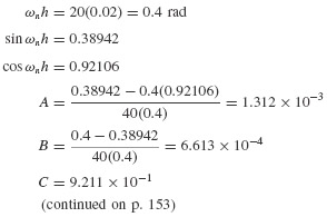
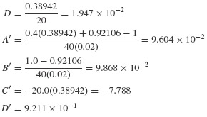
The results are tabulated in Table 1.
Table 1 Numerical Solution Based on Piecewise-Linear Interpolation of the Excitation (Exponent in Parentheses)
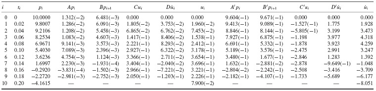
The results are tabulated in Table 1.
(b) The exact solution is given by Eq. 9 of Example 4.1. For discrete times ti this can be written
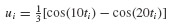
The results are tabulated in Table 2. By comparing the solution based on piecewise-linear interpolation of the excitation with the exact solution, we see that there is good agreement. Since the period of the excitation,
Table 2 Numerical Solution Based on the Exact Response Function (Exponent in Parentheses)
| i | ti |  |
| 0 | 0 | 0 |
| 1 | 0.02 | 1.967(−2) |
| 2 | 0.04 | 7.478(−2) |
| 3 | 0.06 | 1.543(−1) |
| 4 | 0.08 | 2.419(−1) |
| 5 | 0.10 | 3.188(−1) |
| 6 | 0.12 | 3.665(−1) |
| 7 | 0.14 | 3.707(−1) |
| 8 | 0.16 | 3.230(−1) |
| 9 | 0.18 | 2.232(−1) |
| 10 | 0.20 | 7.916(−2) |
is approximately 30 times Δt, the piecewise-linear approximation of cos Ωt should be quite good.
For hand calculation of the response, the tabular form of Table 1 is convenient. Recurrence formulas of the form given in Eqs. 6.7 are easily programmed for a digital computer or programmable calculator.
The next example illustrates how the use of Matlab can provide efficient, easily interpreted implementations of the methods based on exact integration of the governing SDOF equation using either piecewise-constant or piecewise-linear interpolation of the forcing function.1
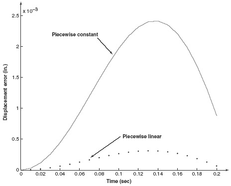
Example 6.2 Comparison of Piecewise-Constant and Piecewise-Linear Algorithms Consider again Example 4.1, where k = 40 1b/in., ωn = 20 rad/sec, and p(t) = 10 cos(10t) 1b. Use Matlab to obtain plots of the response based on piecewise-constant interpolation of the forcing function and the response based on piecewise-linear interpolation of the forcing function.
SOLUTION In Example 6.1 we derived the constants A, B, C, D, A', B', C', and D' that define a simple step-by-step recursion summarized in Eqs. 6.7a and b. This recursion is easy to implement in a few lines of Matlab code. The .m-files that encode the approximation process are:
- mat-ex-6-1.m: Matlab example for piecewise-constant approximation of forcing function
- mat-ex-6-2.m: Matlab example for piecewise-linear approximation of forcing function
- pc-exact-int.m: Matlab function for calculating piecewise-constant exact integration
- plin-exact-int.m: Matlab function for calculating piecewise-linear exact integration
In this example, the time step has been selected to be Δt = 0.01 sec. The right-hand-side function p(t) = 10cos(10t) 1b has been approximated by piecewise-constant and piecewise-linear interpolation of the forcing function. The results are depicted in Figs. 1 and 2. Figure 1 clearly shows that there is little difference between the two methods as to the transient response predicted. Figure 2 shows that the error is on the order of 10−3 for each method.
Figure 1 Response comparison of piecewise-exact integration methods.
Figure 2 Error comparison of piecewise-exact integration methods.
6.1.2 Average Acceleration Method
In Section 6.1.1, recurrence relations based on interpolation of the excitation were obtained. These permit the response of a linear SDOF system to be obtained at discrete times ti. An alternative approach, which may be used for determining the response of both linear and nonlinear systems, is to approximate the derivatives appearing in the system equation of motion and to generate a step-by-step solution using time steps Δti. Although many such procedures are available for carrying out this numerical integration of second-order differential equations (see, e.g., Refs. [6.2] to [6.4]), one of the most common is the Average Acceleration Method,2 which we consider next.
The equation of motion to be integrated is
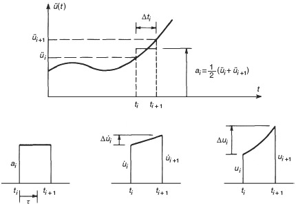
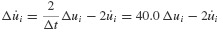
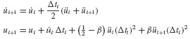
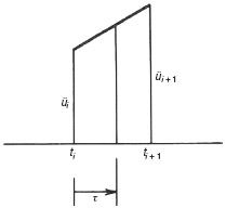
with initial conditions u(0) = u0 and  given. The acceleration is approximated as shown in Fig. 6.3. The acceleration in the time interval ti to ti+1 is taken to be the average of the initial and final values of acceleration, that is,
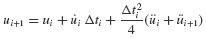
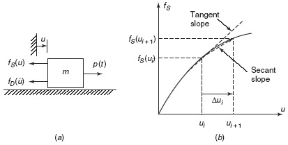
Integration of Eq. 6.9 twice gives
and
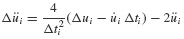
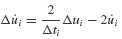
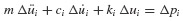
In setting up the computational algorithm for this numerical integration problem, it is convenient to employ previously computed values  and üi, and the incremental quantities Δpi, Δui,
  where Δpi = pi+1 − pi, and so on.3 Then Eq. 6.11 can be solved for Δüi and Eqs. 6.10 and 6.11 combined to give
  as follows:
and
Since Eq. 6.8 is satisfied at both ti and ti+1, we can form the following incremental equation of motion:
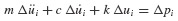
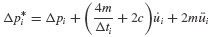
Equations 6.12 through 6.14 can be combined to give the equation

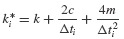
where
and
Once Δui has been determined from Eq. 6.15,  can be obtained from Eq. 6.13 and Δüi from Eq. 6.12, and the updated values of u
  , and üi determined from

The acceleration at time ti can be obtained from the equation of motion,
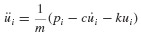
Therefore, üi+1 can be obtained from this equation rather than from Eqs. 6.12 and 6.17c. This equation is also used to obtain ü0.
Figure 6.3 Numerical integration using the Average Acceleration Method.
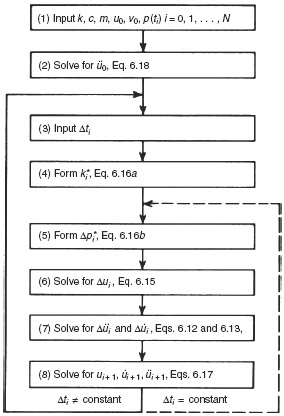
A computational algorithm based on the equations above is summarized in the flowchart shown in Fig. 6.4. If Δti is constant, steps 3 and 4 can be removed from the inner loop. We discuss numerical integration methods further, in Chapter 16, including the Average Acceleration Method.
Figure 6.4 Flowchart for step-by-step numerical integration based on the Average Acceleration Method.
Example 6.3 For the undamped SDOF system in Examples 4.1 and 6.1, use the Average Acceleration Method to determine the response u(t) for 0 ≤ t ≤ 0.2 sec. Use a constant time step Δt = 0.02 sec and also Δt = 0.005 sec. Compare the results with the exact solution of Example 6.1.
SOLUTION From Example 4.1, k = 40 1b/in., c = 0, m = 0.1 1b-sec2/in., ωn = 20 rad/sec, and p(t) = 10cos(10t) 1b. The response results are shown in Table 1.
Table 1 Response u(ti) via the Average Acceleration Method (Exponent in Parentheses)
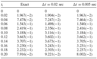
A rule of thumb that Δt should satisfy Δt ≤ T/10, where T is the smallest period in the excitation (see Chapter 16) or the natural period Tn, whichever is smaller, is frequently stated. In Example 6.3 the natural period, Tn = 2π/ωn = 0.314 sec, is smaller than the excitation period, T = 0.628 sec. The time step Δt = 0.02 sec satisfies the rule of thumb and, as seen in Example 6.3, gives satisfactory accuracy. The shorter time step, Δt = 0.005 sec, reproduces the “exact” solution almost identically. Chapter 16 gives further information on the relationship of time step to accuracy of solution.
6.2 INTEGRATION OF FIRST-ORDER ORDINARY DIFFERENTIAL EQUATION
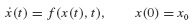
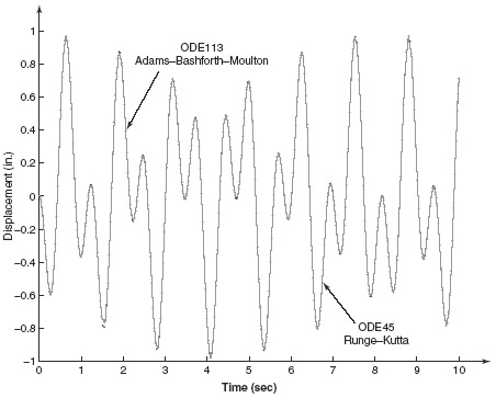
In this section we present several techniques for integration of ordinary differential equations in first-order form. As in Section 6.1, the primary purpose of the chapter is the discussion of numerical methods for approximation of the solution of the prototypical equation of structural dynamics:

The application of the methods in this section require that Eqs. 6.19 be recast in first-order, or state-variable, form. For the second-order system of Eqs. 6.19, the state of the system consists of two variables, the displacement u(t) and the velocity  In this book, we use two distinct first-order differential equations that are equivalent to Eqs. 6.19 referred to as the state-space form and generalized state-space form of the governing equations. The latter form is introduced in Section 10.4 and is applied to experimental structural dynamics in Chapter 18.
To derive the state-space form of the governing equations, a new dependent variable  is introduced.4
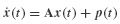
It is easy to see that Eqs. 6.19 are equivalent to the system
where
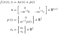
A close inspection of Eq. 6.21a for the case when the underlying second-order ODE is linear, as in Eq. 6.19, reveals that the new first-order equation becomes
Thus, the first-order equation is linear in the state x(t). However, the analysis presented in this section is based on the more general nonlinear form, as given in Eq. 6.21a.
6.2.1 Direct Taylor Series Methods
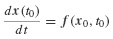
Perhaps the simplest means to achieve numerical integration of the system of first-order ordinary differential equations, Eqs. 6.21, uses the following Taylor series expansion of x(t) in a neighborhood of x0:
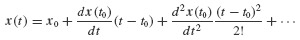
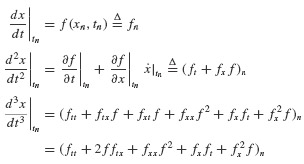
The evaluation of the right-hand side of Eq. 6.24 requires calculation of the derivatives
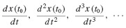
But Eqs. 6.21 can be used to obtain each of these quantities. For example, the first and the second derivatives can be calculated as follows:
By the chain rule of differentiation, we have
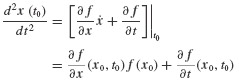
The entries of this equation must be interpreted by context. We have the matrix derivative
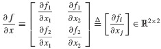
and the vectors
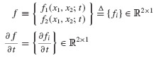
where the subscripts i and j denote the row and column, respectively, of the matrix expressions. Higher-order derivatives can be calculated in an identical manner, although the notation becomes increasingly complex.
Similar Taylor series expansions can be performed at later time steps ti about the current state xi. With this observation, the development of a numerical integration procedure is straightforward. Define the operator Tk,h(x(t), t) to be
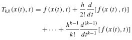
Recall that each of the terms on the right-hand side can be constructed from the chain rule, as in Eq. 6.27. An algorithm to achieve the numerical integration of the governing equations is given in Table 6.2.
Table 6.2 Algorithm for Direct Taylor Series Method
| Step 1 | Choose a partitioning  of the time interval of interest [t0, tN]. of the time interval of interest [t0, tN]. |
| Step 2 | Loop for all the time steps i = 1 … N. |
| h = ti − ti−1 xi = xi−1 + hTk,h(xi−1, ti−1) |
|
| Step 3 | Return to step 2. |
6.2.2 Runge–Kutta Methods
The derivation in the preceding section showed that higher-order accuracy can be obtained, in principle, using the Taylor series approach for integrating first-order ordinary differential equations. However, it is often not practical to evaluate analytically the higher-order derivatives of f on the right-hand side of Eq. 6.28. One of the most popular methods to integrate the equations of motion numerically in first-order form relies on Taylor series approximations but does not require that analytical derivatives be derived for higher-order derivatives. These methods are referred to as the Runge–Kutta methods.
Runge–Kutta Method of Order 2 Runge–Kutta methods include integration formulas of arbitrarily high single-step accuracy. The nature of these methods can be illustrated by considering one of the lower-order versions. Extension to higher-order accuracy follows the same arguments. In the preceding section we studied the vector-valued system of first-order differential equations, Eqs. 6.21. To simplify our notation, we derive the approximate integration methods in the next few sections for the scalar first-order equation

We leave it as an exercise for the reader (Problem 6.12) to show that the discrete integration methods derived for Eqs. 6.29 hold for Eqs. 6.21 with only the straightforward change to vector notation.
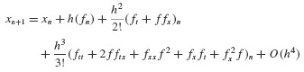
Suppose that we make the assumption that successive approximations xn and xn+1 to the solution x(t) of Eq. 6.29 at times tn and tn+1 are related by the expression

In this expression, the constants c1, c2, c3, and c4 are, as yet, unknown constants that characterize the numerical method. Note that all the right-hand-side terms of Eq. 6.30 can be evaluated once the constants are determined, and (xn, tn) are also known. From our discussion of Taylor series approximations in Section 6.2.1, we can calculate an approximation of xn+1 via

We can write
When we substitute these expressions into the Taylor series in Eq. 6.31, the series becomes
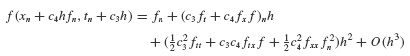
On the other hand, we can expand the last term in Eq. 6.30 in a Taylor series to obtain
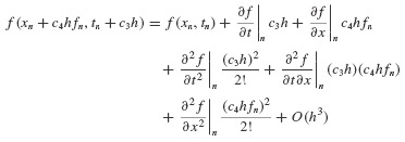
so
Finally, we can substitute Eq. 6.34 into Eq. 6.30, which gives
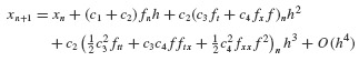
We now compare Eqs. 6.33 and 6.35. The goal is to choose the constants c1, c2, c3, and c4 so that the assumption in Eq. 6.30 is as accurate as possible. That is, we choose the constants so that the expressions match, insofar as this is possible. We see that we must choose
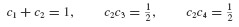
to obtain expressions that match through O(h2). We have obtained three equations in the four unknowns, and it follows that there are many solutions to this system of equations. A review of the literature suggests that the most popular choice of constants is
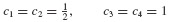
The resulting recursion formula,
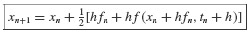
is called the Runge–Kutta Method of Order 2 often referred to as the RK2 Method. Other solutions to Eqs. 6.36 exist, as illustrated by Problem 6.13, but these do not yield the symmetric form of Eq. 6.38.
Example 6.4 Taylor Series and Runge–Kutta Method of Order 2 In this example, we use the Runge–Kutta Method of Order 2 and the Taylor Series Method of Order 2 to approximate the transient response of the SDOF system in Example 4.1. A fixed time step of Δt = 0.001 is used in this simulation. The examples have been written using Matlab, and the .m-files that encode the approximation process are:
- mat-ex-RKO2.m: Matlab example of Runge–Kutta Method of Order 2
- f2ndO1stO.m: a function to convert second-order form to first-order form
- mat-ex-tay.m: Matlab example of Taylor's Method of Order 2
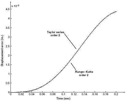
As shown in Fig. 1, the approximations of the transient response provided by these two functions are nearly indistinguishable. Even the error plots in Fig. 2 are nearly overlaid.
Figure 1 Response comparison of second-order Taylor series and RK methods.
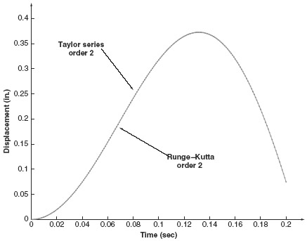
Figure 2 Error comparison of second-order Taylor series and RK methods.
Runge–Kutta Method of Order 4 The general procedure outlined in the preceding section can be carried out to obtain higher-order approximations, but the algebraic manipulations become increasingly tedious. For completeness, we simply note here that perhaps the most popular choice among Runge–Kutta methods is the Runge–Kutta Method of Order 4. At time step n, evaluate the following constants:
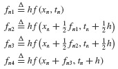
Then the Runge–Kutta Method of Order 4, commonly known as the RK4 Method, uses the following recursion formula:
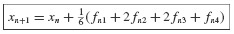
to generate the approximation  to the values of the true solution
In reviewing the Runge–Kutta methods discussed in this section, the following observations should be kept in mind:
- The computational cost of the Runge–Kutta methods is usually summarized in terms of the number of “function evaluations,” that is, evaluations of the right-hand side f(x,t) in one time step of the algorithm.
- The Runge–Kutta Method of Order 2 requires two function evaluations:
at each time step tn to advance to tn+1. Similarly, the Runge–Kutta Method of Order 4 requires four function evaluations at each time step. This is a generic property of all Runge–Kutta methods: the algorithm of order N requires N function evaluations.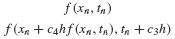
- The Runge–Kutta methods are “self-starting” in the sense that knowledge of the time and state (tn, xn) at time step n is all that is required to progress to the next time step. As we will see in the next section, some techniques require several past values of the time and corresponding state.
6.2.3 Linear Multistep Methods
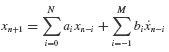
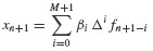
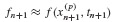
In the Runge–Kutta methods in the preceding section, the propagation of the approximate state from one time step to the next began by using only the current time and state (tn,xn). In contrast, the class of Linear Multistep Methods begin with the assumption that the next approximate state can be written as a linear combination of the states and derivatives at a number of different time steps. That is, the underlying assumption is that
Several observations should be made at this point.
- The name of these methods derives from the assumption that the time propagation expression relies linearly on the past states and functional evaluations. It should be emphasized that the methodology is applicable to nonlinear ordinary differential equations of the general class we are studying in Eqs. 6.21.
- The first summation involves only the past states xn, xn−1, … xn−N, which are known at time step tn.
- The second summation involves the derivatives of the states
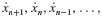
 . Note that
  is unknown, being a future quantity, at time step tn. Thus, if b−1 ≡ 0, the entire right-hand side depends only on past values of the states. This class of methods is known as the explicit, forward, or closed linear multistep methods.
 - On the other hand, if
 the second summation depends on
  This quantity is not known at time step tn. This class of methods is known as implicit, backward, or open linear multistep methods.
Explicit Multistep Methods In general, the derivation of numerical integration methods from Eq. 6.41 begins by integrating the original equation of motion
from tn to tn+1, thereby achieving
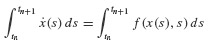
or
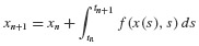
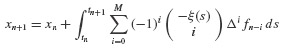
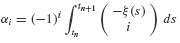
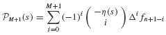
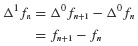
We approximate f(x(s),s) by a polynomial  that interpolates f(x(s),s) at the sequence of points {fn, fn−1, …, fn−M}. It is a classical result of numerical analysis that the approximation will correspond to a polynomial passing through these points provided that we choose
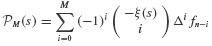
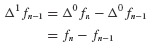
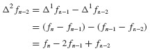
where ξ(t) = (t − tn)/h and Δi is the difference operator that is defined recursively via
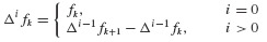
The notation  denotes the binomial function, which is defined by the formula
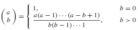
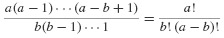
Sometimes the last expression is easier to remember when written in terms of the factorial notation
Equation 6.43 is known as the Newton Backward Formula for the interpolating polynomial of order M passing through the M + 1 points fn, fn−1, …, fn−M. Substitute Eq. 6.43 into Eq. 6.42 to get
or
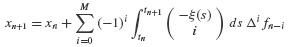
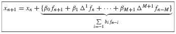
This last expression can be rewritten as
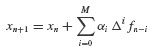
where
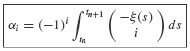
By combining terms, we have found an expression precisely of the form shown in Eq. 6.41.
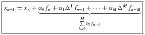
The coefficients  in Eq. 6.41 can be calculated directly from the definition of the difference operator and the coefficients defined in Eq. 6.48. The coefficients can be calculated by hand or by using a symbolic manipulation computer program. Carefully note that all of the terms on the right-hand side of Eq. 6.49 are known at time step tn. Hence, xn+1 can be calculated immediately. This property gives rise to the name of these techniques: Explicit Multistep Methods.
Example 6.5 Adams–Bashforth Method In Section 6.2.2 we derived the Runge–Kutta Method of Order 2, and in Eq. 6.40 we stated the Runge–Kutta Method of Order 4. In this example we develop the form of the Fourth-Order Explicit Linear Multistep Method as defined by Eq. 6.49.
SOLUTION We can directly calculate (or use a symbolic computation program) to obtain the following constants:

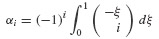
For example, from the definition of αi in Eq. 6.48, we can determine α0,α1,… as follows:
where

By a simple change of variables, the integral can be written as
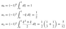
For i = 0, 1, 2, we have

and the corresponding integral expressions are
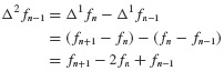
By definition of the difference operators, Eq. 6.44, we have
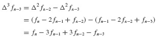
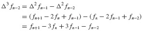
When we substitute the difference formulas above into Eq. 6.49, the following recursion formula is obtained:
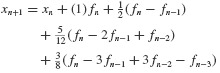
or, in final compact form,
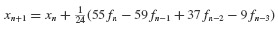
Equation 4 is known as the Adams–Bashforth Method of Order 4.
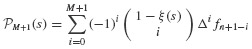
Implicit Multistep Methods Suppose, in contrast to selecting a polynomial  that interpolates the following set of values {fn, fn−1, … fn−M}, we had instead chosen a polynomial
  that interpolates the set of values {fn+1, fn, … fn−M} in Eq. 6.42. Such a polynomial can be written in terms of the backward difference formula introduced in the preceding subsection. Thus, from Eq. 6.43,
where η(t) = (t − tn+1)/h. This equation can be rewritten in terms of the previously introduced function ξ(t) by noting the identity
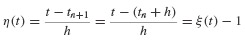
The polynomial  is then
When we substitute this equation into Eq. 6.42, a new expression for the multistep formula is obtained:
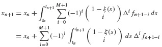
or
where
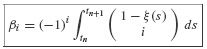
In other words, we have derived a multistep formula that has the form
The coefficients  can be calculated by hand or by using a symbolic calculation program. In comparing the summation above to the explicit multistep formulas of the preceding section, it is important to note that the summation above includes the term fn+1, which is not known at time step n. This term gives rise to the name of these techniques: Implicit Multistep Methods.
Example 6.6 Adams-Moulton Method In Example 6.5 we derived an explicit fourth-order multistep method known as the Adams-Bashforth Method. In this example, we derive a corresponding fourth-order multistep method that is implicit.
SOLUTION We can show that the constants βi given by Eq. 6.53, are

By definition of the difference operators, Eq. 6.44, we have
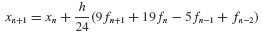
The Adams–Moulton Method is defined by substituting the definitions above into the implicit multistep formula, Eq. 6.54. Then
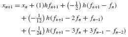
Finally,
Overview of First-Order Numerical Integration In summary, then, we can make the following general observations that will guide us in the selection of an integration method introduced in Section 6.2 for first-order ordinary differential equations.
- The Direct Taylor Series Method provides a good theoretical foundation and conceptual bridge to more advanced methods.
- The Direct Taylor Series Method is seldom used in practice. The right-hand-side function f(x(t), t) must be simple to differentiate to use this method in applications.
- Runge–Kutta methods have the generic advantage that they are self-starting. That is, only the state at the current time step is required to propagate a numerical approximation of the state at the next time step.
- Runge–Kutta methods measure their computational costs in terms of the number of evaluations of the right-hand-side function f(x(t), t) at each time step.
- Runge–Kutta Methods of Order K require K evaluations of the function f(x(t), t) at each time step.
- Linear Multistep Methods are not, generally speaking, self-starting.
- Explicit Linear Multistep Methods of Order K require one evaluation of the function f(x(t), t) per time step.
- Explicit Linear Multistep Methods of Order K require the storage of roughly (K − 1) previous evaluations of the function f(x(t), t) at each time step.
In general, the Runge–Kutta methods are often preferred because they are self-starting. For very long simulations, however, the Linear Multistep Methods can be more efficient. The most popular variants of these methods use error estimators to adapt the time step size or the order of the method to achieve a given accuracy. Other popular techniques combine the Explicit and Implicit Multistep Methods to create Predictor–Corrector Methods. These topics are beyond the scope of this book. The interested reader is referred to Refs. [6.5] to [6.8].
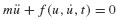
Both of the numerical approaches summarized in Sections 6.1 and 6.2, those derived for second- and first-order ODEs, can be useful in approximating the response of nonlinear systems. Before considering the numerical solution of the nonlinear equation of motion, let us consider some of the physical phenomena that lead to nonlinearities in the equation of motion of a SDOF system.5 The equation of motion of a linear SDOF system is, of course,
The equation of motion of a nonlinear SDOF system can often be written in the form
Since this is not a linear differential equation, the principle of superposition does not hold. Thus, for example, the Duhamel integral cannot be used to obtain the solution for the nonlinear response u(t).
In Section 4.7 it was indicated that damping can lead to nonlinear terms in the equation of motion and that equivalent viscous damping may sometimes be employed to approximate the actual nonlinear damping in a system. The damping force of a fluid acting on an object moving through it, and Coulomb damping, were cited as common nonlinear damping mechanisms. Two important classes of nonlinearities related to the displacement u(t) are geometric nonlinearity and material nonlinearity. These will be illustrated briefly.
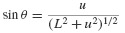
Consider the taut string (neglect bending) with attached lumped mass m shown in Fig. 6.5. The tension in the string is given by

where T0 is the tension in the undeflected string and δ is the elongation of the string given by
From the free-body diagram in Fig. 6.5, the equation of motion is found to be

or
But
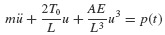
Thus, the nonlinear equation of motion is
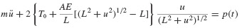
This exact nonlinear differential equation has the form of Eq. 6.56, with the nonlinear term being a geometric nonlinearity; that is, the nonlinearity depends only on geometric quantities, length and displacement, and not on any material properties. For “small” displacements, that is, u « L, Eq. 6.62 can be approximated by the linear equation
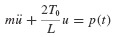
For somewhat larger displacements,
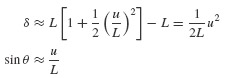
so Eq. 6.62 can be approximated by
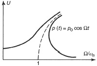
The cubic term in Eq. 6.64, preceded by a plus sign, leads to what is referred to as a hardening spring. Under harmonic excitation such a system exhibits a frequency-response behavior characterized by the solid curves in Fig. 6.6. The dashed curve in Fig. 6.6 represents the locus of resonant frequencies, indicating that the resonant frequency increases with increasing amplitude of response. Note also that at some values of Ω/ωn, three different amplitudes are possible. References [6.9], [6.10], and others give detailed studies of the response of systems with a hardening or softening spring to harmonic excitation.
Figure 6.5 Large deflection of a mass on a taut string.
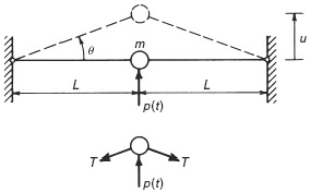
Figure 6.6 Frequency-response curve for a SDOF system with a hardening spring.
Next, let us consider an example of a material nonlinearity. Figure 6.7a represents an idealized steel frame whose columns are assumed to be much more flexible than the horizontal “roof member”. If the load p is increased slowly, the load-deflection curve of Fig. 6.7b results. The load–deflection behavior is linear up to point B, where yielding begins at the outer fibers at the points labeled “plastic hinges,” where the moment is the greatest. The load is increased further to point C. Thereafter the load is reduced, and the load-deflection curve from C to E follows a straight line parallel to the original
Figure 6.7 (a) Steel frame under loading that produces yielding of columns; (b) load-deflection diagram.
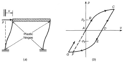
slope of portion AB. At point D the direction of loading is reversed. The closed loop ACFA is called a hysteresis loop. The area inside the loop is the energy dissipated as a result of cyclic plastic deformation. The force–displacement relationship of Fig. 6.7b and other models of structural nonlinearities are discussed in Refs. [6.11] to [6.13]. A simpler model, the elastic–perfectly plastic model, is illustrated in Example 6.8 in Section 6.3.2.
6.3.1 First-Order Formulation of Nonlinear SDOF Systems
The numerical approximation methods derived for first-order ordinary differential equations are directly applicable to the simulation of the response of geometrically nonlinear SDOF systems. For example, the prototypical equation of motion for many nonlinear SDOF systems can be written as
with initial conditions
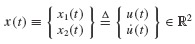
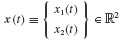
Just as in our study of linear SDOF systems, the nonlinear equation of motion can readily be converted to first-order form. We define a state vector

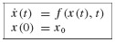
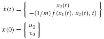
The corresponding first-order equation of motion has the form
Then Eqs. 6.65 and 6.66 take the state-space form
We have studied several methods for approximating the transient response of systems having this form. These methods include, for example, the family of Runge–Kutta Methods and the family of Multistep Methods.
In Sections 6.2.2 and 6.2.3 we derived the fourth-order Runge–Kutta Method, fourth-order (Explicit) Adam–Bashforth Multistep Method, and fourth-order (Implicit) Adams–Moulton Multistep Method. The Runge–Kutta and Multistep Methods are so popular that nearly all commercially available numerical integration packages contain some representatives of these classes. In particular, Matlab has several built-in functions that encode Runge–Kutta and Multistep Methods. In Example 6.7 we show how to use the general framework that has been constructed by the authors of Matlab to employ their numerical integration packages. Of course, we cannot present the architecture of the Matlab integration libraries in all their generality. The interested reader is referred to the numerous texts that provide details of the Matlab environment.
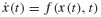
Example 6.7 Runge–Kutta and Multistep Methods for Nonlinear Response In this example we illustrate the use of two specific functions in Matlab:ODE45 and ODE113. If the reader understands how these two standard packages in Matlab can be used to integrate ordinary differential equations, it will be clear how to use many of the other numerical integration algorithms in the Matlab package.
This example computes a simulation of the response of the string-mass geometrically nonlinear system depicted in Fig. 6.5. The Matlab. m-files that have been written to approximate the transient response of this system include:
- mat-ex-6-4.m: the master .m-file that invokes the Matlab built-in functions ODE45 and ODE113 to obtain the solution via two different integration methods
- geomnon.m: an .m-file that returns the nonlinear function f(x(t), t) that is defined in the equations of motion having the form
- geomnon-forcing.m: an .m-file that returns the right-hand-side forcing function acting on the string–mass system at time t
The computed response u(t) is plotted in Fig. 1.
Figure 1 Response based on Runge–Kutta of Order 4 and Multistep Methods.
6.3.2 Second-Order Formulation of Nonlinear SDOF Systems
Incremental, or step-by-step, procedures are the foundation of those numerical integration methods that work directly with the second-order form of the governing nonlinear ordinary differential equations. Most of these methods have a similar philosophy, so that the derivation of a single representative from this class yields a good background for understanding the overall incremental formulation.
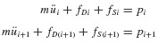
As an example, the average acceleration procedure employed in Section 6.1.2 for determining the response of linear systems may be adapted for determining the response of nonlinear systems. Figure 6.8a shows an SDOF system with possible nonlinear “spring” and “damping” elements. Figure 6.8b illustrates a typical nonlinear force–displacement curve for fS expressed as a function of displacement u. It is assumed that the mass remains constant, although this could easily be generalized to be a known function of time. (The symbols fS and fD will be used whether referring to functions of time or to functions of displacement and velocity.) Then the equation of motion may be written at times ti and ti+1 = ti + Δti as follows:
Subtracting Eq. 6.71a from Eq. 6.71b, we get
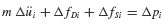
where
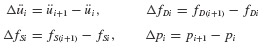
Equation 6.72 differs from Eq. 6.14, which was used in the step-by-step integration algorithm, only in the nonlinear fD and fS terms. An approximation to the ΔfSi term is

where kt is the tangent slope at ut as shown in Fig. 6.8b. Similarly, an approximation to the fD term can be written in the form

where ci is the tangent slope of the fD versus u curve at  . Then Eq. 6.72 becomes
This replaces Eq. 6.14 in the step-by-step integration algorithm of Section 6.1.2. Thus, the response of a nonlinear system can be computed using the steps outlined in the flowchart of Fig. 6.4, with c and k being replaced by ct and kt evaluated at the beginning of each time step. By using Eq. 6.71b to compute the acceleration at the end of the present time step (and the beginning of the next time step), dynamic equilibrium is enforced at each time step. Due to the approximations in Eqs. 6.74, if üi were computed using Eqs. 6.12 and 6.17c, dynamic equilibrium would not be satisfied at time ti+1 unless c and k remained constant over the time step. In general, the time step Δti must be small enough that the difference in a linear solution and nonlinear solution over one time step is not great.
Figure 6.8 (a) Nonlinear SDOF system; (b) force–deformation curve.
The following example illustrates the use of the average acceleration step-by-step integration algorithm for calculating the response of a nonlinear SDOF system.
Example 6.8 The frame shown in Fig. 6.7a has an elastic, perfectly plastic force-deformation behavior, as shown in Fig. 1a. This is an idealization of the behavior
Figure 1 (a) Elastic–plastic material behavior and (b) rectangular pulse loading history for the elastic–plastic frame example.
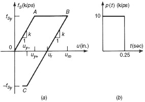
shown in Fig. 6.7b. The frame, with m = 0.2 kip-sec2/in., k = 30 kips/in. (total), and fsy = 15 kips, is subjected to a rectangular pulse loading as shown in Fig. 1b. Compare this problem with the corresponding linear problem in Section 5.2. The frame is at rest at t = 0. Use the Average Acceleration Method to compute the response u(t) for t = 0 to t = 0.55 sec. Use Δt = 0.05 sec (constant).
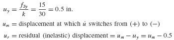
SOLUTION The flowchart of Fig. 6.4 can be adapted by using the following equations:
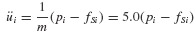
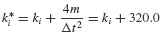
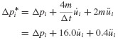

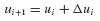

For the present problem, ki has the value k = 30 kips/in. or zero depending on the deformation history. Other relevant values are:
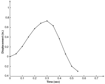
Tables 1 and 2 outline the calculation of the response of the elastic-plastic system and of an elastic system (assuming that fy > max|fs|, i.e., ignoring yielding) using the average acceleration algorithm. Figure 2 shows the elastic–plastic response.
Table 1 Numerical Solution for Elastic–Plastic Response Calculated by the Average Acceleration Method
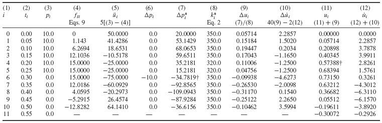
Table 2 Numerical Solution for Elastic Response Calculated by the Average Acceleration Method
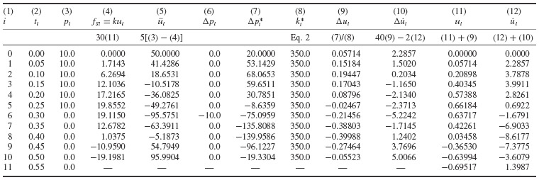
Figure 2 Material nonlinearity: response with elastic-plastic behavior.
In Tables 1 and 2, note that the expressions for  and fSi change at the †-symbols; first, where ut first exceeds uy, and next, where
  changes sign. If the computations were to continue, a further change would be required.
Example 6.8 illustrates briefly the complex nature of numerical solution of nonlinear structural dynamics problems. Numerical solution of nonlinear MDOF problems is discussed briefly in Section 16.3.3.
REFERENCES
[6.1] R. W. Clough and J. Penzien, Dynamics of Structures, 2nd ed., McGraw-Hill, New York, 1993.
[6.2] N. M. Newmark, “A Method of Computation for Structural Dynamics,” Transactions of ASCE, Vol. 127, Pt. 1, pp. 1406–1435, 1962.
[6.3] K. J. Bathe and E. L. Wilson, “Stability and Accuracy Analysis of Direct Integration Methods,” Earthquake Engineering and Structural Dynamics, Vol. 1, pp. 283–291, 1973.
[6.4] H. M. Hilber, T. J. R. Hughes, and R. L. Taylor, “Improved Numerical Dissipation for Time Integration Algorithms in Structural Dynamics,” Earthquake Engineering and Structural Dynamics, Vol. 5, pp. 283–292, 1977.
[6.5] C. W. Gear, Numerical Initial Value Problems in Ordinary Differential Equations, Prentice-Hall, Englewood Cliffs, NJ, 1973.
[6.6] A. Ralston and P. Rabinowitz, A First Course in Numerical Analysis, McGraw-Hill, New York, 1978.
[6.7] S. D. Conte and C. de Boor, Elementary Numerical Analysis: An Algorithmic Approach, McGraw-Hill, New York, 1980.
[6.8] T. J. R. Hughes, The Finite Element Method: Linear Static and Dynamic Finite Element Analysis, Dover, New York, 2000.
[6.9] J. J. Stoker, Nonlinear Vibration, Wiley, New York, 1950.
[6.10] W. J. Cunningham, Introduction to Nonlinear Analysis, McGraw-Hill, New York, 1958.
[6.11] M. A. Sozen, “Hysteresis in Structural Elements,” Applied Mechanics in Earthquake Engineering, AMD Vol. 8, ASME, New York, pp. 63–98, 1974.
[6.12] A. K. Chopra, Dynamics of Structures: Theory and Applications to Earthquake Engineering, 2nd ed., Prentice Hall, Upper Saddle River, NJ, 2001.
[6.13] G. C. Hart and K. Wong, Structural Dynamics for Structural Engineers, Wiley, New York, 2000.
PROBLEMS
For problems whose number is preceded by a C, you are to write a computer program and use it to produce the plot(s) requested. Note: Matlab .m-files for many of the plots in this book may be found on the book's website.
Problem Set 6.1
6.1 For the undamped SDOF system in Example 4.1, determine the response u(t) for 0 ≤ t ≤ 0.4 s. Use piecewise-constant interpolation of the force, with the magnitude of each impulse determined by the force at the beginning of each time step Δt = 0.02 s (Fig. P6.1).
6.2 Repeat Problem 6.1, but with the magnitude of each impulse being determined by the force at the middle of each time step Δt = 0.02 s.
6.3 Repeat Problem 6.1, but with the magnitude of each impulse being determined by the force at the end of each time step Δt = 0.02 s.
6.4 (a) Repeat part (a) of Example 6.1, but double the time step to Δt = 0.04 s. (b) Tabulate your results from part (a), and compare them with the exact solution and with the numerical solution of Problem 6.1.
C 6.5 Write a Matlab program to approximate the response u(t) for the undamped system in Example 4.1. Use the numerical integration technique derived in Problem 6.1. Choose the time step to be an input variable Δt, and select Δt = 0.02 s in the simulation. Plot your result u(t) versus t.
C 6.6 Write a Matlab program to approximate the response u(t) for the undamped system in Example 4.1. Use the numerical integration technique derived in Problem 6.2. Choose the time step to be an input variable Af, and select Δt = 0.02 s in the simulation. Plot your result u(t) versus t.
C 6.7 Write a Matlab program to approximate the response u(t) for the undamped system in Example 4.1. Use the numerical integration technique derived in Problem 6.3. Choose the time step to be an input variable Δt, and select Δt = 0.02 s in the simulation. Plot your result u(t) versus t.
C 6.8 Repeat the numerical simulations in Problems 6.5, 6.6, and 6.7 with the selection of time steps sizes Δt = 0.1, 0.2, 0.3, and 0.4 s, respectively. For each integration method (derived in Problems 6.5, 6.6, and 6.7, respectively), create a graph that contains four plots of error versus time for each of the time following time steps: Δt = 0.1, 0.2, 0.3, and 0.4 s.
6.9 The Newmark β method, referred to in footnote 1 in Section 6.1.2, is embodied in the equations
(a) Show that  corresponds to the Linear Acceleration Method, wherein the acceleration approximation in Fig. 6.3 is replaced by the linear interpolation shown in Fig. P6.9. (b) Determine expressions for
  and
and  for the Linear Acceleration Method similar to those for the Average Acceleration Method as given by Eqs. 6.16a and b.
6.10 Repeat Example 6.3 using the Linear Acceleration Method as derived in Problem 6.9 instead of the Average Acceleration Method.
C 6.11 Write a Matlab program that encodes the New-mark β Method for a constant input time step Δt and fixed input choice of β. Obtain a numerical approximation to Example 6.3 using the Linear Acceleration Method (i.e.,  .
.
Problem Set 6.2
6.12 In the text we noted that the numerical integration methods we derived for the first-order scalar ordinary differential equation,

can be implemented without change, except notation, to systems of ordinary differential equations having the (vector) form

Argue that this is true. Start with a simple low-dimensional system. Choose, say,
Extend your argument to higher dimensions.
6.13 In Section 6.2.2 the Runge–Kutta Method of Order 2 was derived, and a popular selection for the four constants is given in Eq. 6.37. The resulting recursion formula is given in Eq. 6.38. (a) Determine an alternative set of constants if c = ¼ is one of them. (b) What is the resulting recursion formula?
C 6.14 Repeat Example 6.4, but generate a comparison of the accuracy of (a) the Runge–Kutta Method of Order 2, (b) the Taylor Series Method of Order 2, and (c) the Runge–Kutta Method of Order 4 as the time step varies from Δt = 0.001 to Δt = 0.0001.
6.15 Explicit and Implicit Multistep Methods are frequently used in tandem to generate Predictor–Corrector Methods. First, an explicit method is used to generate a prediction of the state at the next time step, denoted  from Eq. 6.49. Next, correction of the approximate value of the state at the next time step
  is generated from Eq. 6.54. The unknown function evaluation fn+1 in Eq. 5 of Example 6.6 is approximated by the evaluation
Using the results from Examples 6.5 and 6.6, write a detailed flowchart for the fourth-order Adams–Bashforth–Moulton Predictor–Corrector Algorithm. This algorithm is the specific predictor–corrector method that uses the explicit Adams–Bashforth formula in the prediction phase of the algorithm and uses the implicit Adams–Moulton formula during the correction phase.
Problem Set 6.3
C 6.16 Write an Adams–Bashforth–Moulton Predictor–Corrector Algorithm in Matlab as it is outlined in Problem 6.15. Repeat Example 6.7 using the fixed-time-step predictor–corrector algorithm that you have written. Compare the consistency of this fixed-time-step method with the adaptive time step (and adaptive order) Runge–Kutta and Adams–Bashforth–Moulton Methods that are encoded in the built-in Matlab integration functions ODE45 and ODE113, respectively.
6.17 Repeat Example 6.8 using the Linear Acceleration Method as derived in Problem 6.9 instead of the Average Acceleration Method.
1 The Matlab. m-files that are listed in Examples 6.2, 6.4, and 6.6 may be found on the book's website.
2 This method is also referred to as the Newmark  Method, the Trapezoidal Rule, and the Constant-Average-Acceleration Method.
3 The incremental form presented here is used in the nonlinear analysis of Section 6.3.2. An alternative “operator formulation” is presented in Chapter 16.
4 It is an accepted practice to use the symbol  to denote the set of all real numbers, and vectors of length N whose elements are extracted from are denoted as belonging to
5 References [6.9] to [6.11] and many other references are available which go into far greater detail on nonlinear structural dynamics than is possible within the scope of this book. References [6.12] and [6.13], in particular, treat nonlinearities in structures subjected to earthquakes.