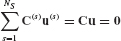
Component-Mode Synthesis
In Chapter 14 you were introduced to finite element techniques for formulating MDOF models of structures for use in structural dynamics analyses. Stiffness and mass matrices were derived for finite elements, and these were assembled to form system matrices. In Section 14.6, general techniques were introduced for reducing the order of system matrices by the use of assumed modes and constraint equations, and Guyan–Irons Reduction was illustrated in Section 14.8. In the present chapter, a class of model-reduction methods known as component-mode synthesis (CMS), or substructure coupling for dynamic analysis, is introduced. Substructuring involves dividing the structure into a number of substructures, or components (e.g., Fig. 17.1), obtaining reduced-order models of the components, and then assembling a reduced-order model of the entire structure.
Figure 17.1 Typical space vehicle substructures: (a) vehicle components; (b) primal assembly; (c) dual assembly. (These figures, which are based on ESA/ESTEC models, are used with the permission of D. J. Rixen, d.j.rixen@wbmt.tudelft.nl.)

CMS methods have been found to be very useful in solving very large structural dynamics problems, especially where the structure consists of several natural components, for example, body and frame components of an automobile, or the space shuttle orbiter and its payloads. Recently, a multilevel substructuring version of component-mode synthesis has been developed for carrying out eigensolutions and frequency-response solutions based on ultralarge finite element models (e.g., finite element models having several million degrees of freedom).
In this chapter we define and illustrate many of the terms that are found in the CMS literature (fixed-interface modes, free-interface modes, constraint modes, residual flexibility, etc.); discuss general procedures for coupling substructures; and discuss several specific CMS methods, including multilevel substructuring.
Upon completion of this chapter you should be able to:
- Obtain, using a finite element model of a simple structural component, component modes of the following types: free-interface normal modes, fixed-interface normal modes, rigid-body modes, constraint modes, attachment modes, residual attachment modes, residual inertia-relief attachment modes.
- Assemble the reduced-order system matrices
 and
and  using the generalized component coupling procedures of Section 17.5.
 - Discuss the importance of including attachment modes when free-interface normal modes are used as the basis for component-mode synthesis.
17.1 INTRODUCTION TO COMPONENT-MODE SYNTHESIS
When a large, complex structural system must be analyzed for its response to dynamic excitation, some form of substructure coupling method, or component-mode synthesis (CMS) method, is usually employed. The term component modes is used to signify Ritz vectors, or assumed modes, that are used as basis vectors in describing the displacement of points within a substructure, or component. Component normal modes, or eigenvectors, are just one class of component modes. In the mid-1960s Hurty published several reports and papers on substructure coupling using fixed-interface modes (e.g., Refs. [17.1] and [17.2]). In collaboration with Hurty, Bamford created a CMS computer program that employed normal modes, rigid-body modes, constraint modes, and attachment modes.[17.3] A simplification of Hurty’s method was presented by Craig and Bampton in 1968[17.4], and in the 1970s MacNeal[17.5], Rubin[17.6], Hintz[17.7], and Craig and Chang[17.8] introduced free-interface methods. A number of CMS methods are described and compared in Refs. [17.9] and [17.10] and in at least three textbooks (Refs. [17.11] to [17.13]). Damping is most often treated as modal damping imposed on the modes of the reduced-order system model. Although special CMS methods have been developed for systems with general viscous damping (e.g., Refs. [17.14] to [17.16]), these methods are not widely used, and therefore they are not discussed in this book.
Component-mode synthesis involves three basic steps: division of a structure into components, definition of sets of component modes, and coupling of the component-mode models to form a reduced-order system model. The primary uses of dynamic substructuring are (1) to couple reduced-order models of moderately complex structures (e.g., space vehicle components, as in Fig. 17.1), (2) in test verification of finite element models of components, or (3) to implement computation of the dynamics of very large finite element models (e.g., multimillion-DOF models). In this chapter we address primarily applications of the first type. References [17.17] to [17.19] illustrate the relationship of substructure analysis to substructure testing, and Refs. [17.20] to [17.22] are representative of the third application, multilevel substructuring.
The most general type of substructure, or component, is one that is connected to one or more adjacent components by redundant interfaces. Figure 17.2 illustrates a simple cantilever beam that is divided into three components; the middle one is a typical component with redundant interface (boundary) coordinates.
Figure 17.2 (a) Typical components and coupled system; (b) coordinate notation for typical component with redundant boundary.

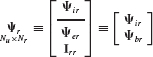
As noted in Fig. 17.2, the coordinate sets  and
and  denote interior coordinates (i.e., not shared with any adjacent component), rigid-body coordinates, excess boundary coordinates (i.e., redundant boundary coordinates), and boundary coordinates (i.e., shared with adjacent components). If a load is prescribed at an “interior” DOF, this DOF can be relabeled as a “boundary” DOF. This is done to permit static completeness of the boundary-coordinate set. The numbers of displacement coordinates in these sets are Ni(s) , Nr(s), Ne(s), and Nb(s), respectively, with Nb(s) = Nr(s) + Ne(s) and Nu(s) = Ni(s) + Nb(s) , where the superscript s is the label of the particular component.
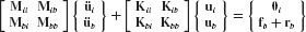
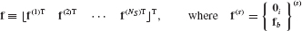
The equation of motion of a typical undamped component, labeled superscript s, may be written as

where M(s), K(s), and u(s) are the component’s mass matrix, stiffness matrix, and displacement vector, respectively, in original physical coordinates. The force vector f(s) contains the externally applied forces, and the force vector r(s) contains the reaction forces on the component due to its connection to adjacent components at boundary degrees of freedom.
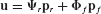
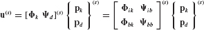
In component-mode synthesis, the component’s physical displacement coordinates u are represented in terms of component generalized coordinates p by the Ritz coordinate transformation

where the component-mode matrix  is a coordinate transformation matrix of preselected component (assumed) modes, including modes of the following types: rigid-body modes, normal modes of free vibration (i.e., eigenvectors), constraint modes, and attachment modes. In collaboration with Hurty, Bamford defined all four of these types of modes.[17.3] Other types of assumed modes (e.g., Krylov vectors[17.23]) may also be employed as component modes.
The coordinate transformation relating component physical coordinates u(s) to component generalized coordinates p(s) is given by Eq. 17.2. This equation, together with the equation of motion in generalized coordinates, forms the component modal model. From Eqs. 17.1 and 17.2, the component equation of motion in generalized coordinates is

where the component mass matrix, stiffness matrix, and force vectors in component generalized coordinates are, respectively,

In Sections 17.2 through 17.4, the systematic procedures used to generate FE-based component modes are described. Section 17.5 presents Lagrange-multiplier-based generalized substructure coupling procedures. This is followed, in Section 17.6, by a discussion of CMS methods that are based on fixed-interface modes, and in Section 17.7, by a discussion of CMS methods based on free-interface modes. Finally, Section 17.8 introduces briefly the concept of multilevel substructuring.
17.2 COMPONENT MODES: NORMAL, CONSTRAINT, AND RIGID-BODY MODES
The following partitioned forms of Eq. 17.1 will be useful in the derivation of component modes, first, where all boundary coordinates are kept as one set ub:
and second, where the boundary coordinates are separated into rigid-body coordinates ur and excess boundary coordinates ue:

Interior forces fi are omitted here, since, as noted previously, DOFs with external loads are assumed to be labeled as boundary DOFs. The coupling force r is discussed in Section 17.5, where coupling procedures are discussed.
The superscript s, which was used in Section 17.1 to designate a typical component, is omitted from component matrices and vectors in this section and in Sections 17.3 and 17.4, but will return later in the discussion of coupling of substructures in Sections 17.5 through 17.7.
17.2.1 Normal Modes
Component normal modes are eigenvectors and may be classified according to the interface boundary conditions specified for the component: fixed-interface normal modes, free-interface normal modes, hybrid-interface normal modes, or loaded-interface normal modes.
Component fixed-interface normal modes are obtained by restraining all boundary DOFs and solving the following eigenproblem:

The complete set of Ni fixed-interface (flexible) normal modes from Eq. 17.7 is labeled Φii and assembled, according to the partitioning of Eq. 17.5, as columns of the modal matrix

When normalized with respect to the mass matrix Mii, the Ni fixed-interface modes satisfy

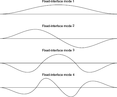
Figure 17.3 shows the four (i.e., Ni) fixed-interface normal modes for the 8-DOF free-free beam component in Fig. 17.2b.
Figure 17.3 Component fixed-interface modes.
A second type of component normal mode used in CMS is the set of free-interface normal modes. These normal modes are defined by the equation

The assembled set of Nf flexible (i.e., non-rigid-body) free-interface normal modes is
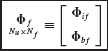
Figure 17.4 shows the first four of the six free–free flex modes of the 8-DOF component in Fig. 17.2b. Note that for this symmetric component, these modes are called the first symmetric mode (mode 1), the first antisymmetric mode (mode 2), the second symmetric mode (mode 3), and so on.
Figure 17.4 Flex modes for the free–free component.

A third important type of component normal modes is loaded-interface normal modes. This includes lumped-mass loaded-interface normal modes, commonly referred to as mass-additive normal modes, which have been employed in modal testing of substructures.[17.17, 17.18] Benfield and Hruda described CMS methods based on “consistent” mass-additive and stiffness-additive normal modes[17.24], but these methods require reduced-order models of all adjacent substructures, so they are generally of limited practical value.
17.2.2 Constraint Modes and Rigid-Body Modes
A constraint mode is defined as the static deformation of a structure when a unit displacement is applied to one coordinate of a specified set of “constraint” coordinates, C, while the remaining coordinates of that set are restrained, and the remaining degrees of freedom of the structure are force-free.
The set of interface constraint modes based on unit displacement of the boundary coordinates ub is a very useful CMS set, because of the ease of enforcing intercomponent compatibility when these constraint modes are employed, as explained in Section 17.6. This set, with  , is given by
That is, the interface constraint-mode matrix  c is given by
From Eqs. 17.8 and 17.12 it can easily be shown that these constraint modes are stiffness-orthogonal to all of the fixed-interface normal modes; that is,

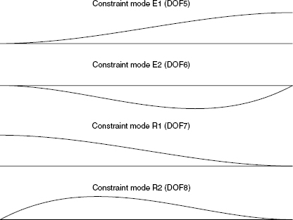
Figure 17.5 shows the Nb (four) constraint modes for the 8-DOF free–free beam component in Fig. 17.2b.
Rigid-body modes can be defined relative to any set of Nr coordinates that is just sufficient to restrain rigid-body motion of the component. A rigid-body mode is an undeformed configuration of a component obtained by setting one of a designated set  of displacements equal to unity, with all of the rest of this set equal to zero, and with
Figure 17.5 Component constraint modes.
all forces on the component equal to zero. (This requires that the stiffness matrix K be singular.) Although they are often considered to be zero-frequency normal modes, rigid-body modes are also a special case of (static) constraint modes.
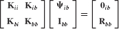
For the purpose of substructure coupling, rigid-body modes will be defined relative to a set of boundary coordinates. Then
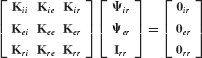
so the set of rigid-body modes is obtained by solving the top two row partitions of Eq. 17.15, giving
where

is the cantilever flexibility matrix for the component restrained at the coordinates, but nowhere else.
Redundant-interface constraint modes can then be defined for unit displacements at the redundant (excess) boundary coordinate set  and with the coordinates fixed, by the equation
Therefore, the set of redundant-interface constraint modes is given by

Either the set of interface constraint modes c defined by Eq. 17.13, or the combined set [r e] defined by Eqs. 17.16 and 17.19, spans the static response of the substructure to interface loading and allows for arbitrary interface displacements ub. Along with the prescribed interface displacement, there is accompanying displacement of the interior of the substructure, as determined by Eqs. 17.13, 17.16, and 17.19. Additional interior flexibility can be incorporated by including fixed-interface normal modes, fixed-interface Krylov vectors, or other fixed-interface assumed modes in the component mode matrix , as illustrated in Section 17.6.[17.2,17.4,17.23]
17.3 COMPONENT MODES: ATTACHMENT AND INERTIA-RELIEF ATTACHMENT MODES
Whereas constraint modes and rigid-body modes are defined by specifying a unit displacement at one DOF, attachment modes are defined by specifying a unit force at one DOF.
17.3.1 Attachment Modes
An attachment mode is defined as the component displacement vector due to a single unit force applied at one of the coordinates of a given set  . Consequently, attachment modes are just columns of the associated flexibility matrix. Attachment modes were defined by Bamford[17.3], and they get their name from their usefulness in representating the deformation of a structure to loading at the point where the attachment mode’s unit force is applied (e.g., an external force, an attached mass, or an attached flexible component). In the present CMS context, we are interested in defining attachment modes to permit statically complete representation of the response of a component to forces at its interface with adjoining components.[17.7, 17.8]
One difficulty encountered in using attachment modes is that many components have one to six rigid-body degrees of freedom, making it impossible to apply directly to the unrestrained component the necessary unit forces in order to compute the resulting attachment mode shapes. However, one option in this case is to select a set of boundary rigid-body degrees of freedom, (mathematically) restrain the component at these DOFs, and then form cantilever attachment modes by applying unit loads at the redundant boundary coordinates, that is, for  . Then

It can be seen that these attachment modes are just an expanded form of the columns of the right-hand partition of the flexibility matrix Gc of Eq. 17.17, with . That is, the cantilever attachment modes are given by
Two important topics that arise when attachment modes are to be employed to represent, in part, the flexible behavior of unrestrained components are inertia relief and residual flexibility. These two topics, and the related forms of attachment modes, are defined in Sections 17.3.2 and 17.4, respectively.
17.3.2 Inertia-Relief Attachment Modes
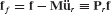
When free-interface normal modes are to be employed in coupling reduced-order components that have rigid-body freedom, it is essential to complement the truncated set of free-interface normal modes with a set of inertia-relief attachment modes that are based on unit forces applied at all boundary coordinates. The term inertia relief refers to the process of applying to the component a self-equilibrated force system ff, which consists of the original force vector f equilibrated by the rigid-body d’Alembert force vector (−Mür), where ur is the rigid-body motion due to f.
Starting with Eq. 17.1, let the displacement vector u be separated into its rigid-body displacement component and its flexible-body displacement component, and expressed in terms of the respective modal coordinates pr, and pƒ. That is, let
where all of the Nƒ flexible-body normal modes are included in Φf. Then the equations

are the appropriate orthogonality equations and the definition of the rigid-body modal mass matrix, respectively. (Note that it is not assumed that the rigid-body modes are mass-normalized, although they may be.) Since (from Eq. 17.15) Kψr = 0, Eqs. 17.1 and 17.22 can be combined to give

When this equation is premultiplied by ψrT and orthogonality is invoked, we can solve for the rigid-body modal acceleration vector,  r, and then form the self-equilibrated force vector
where Pr is the inertia-relief projection matrix, defined by

When any force vector is premultiplied by this inertia-relief projection matrix, the resulting force system is self-equilibrated. Also, from Eq. 17.26 it can easily be verified that PrT is mass-orthogonal to the rigid-body modes; that is,

An important type of inertia-relief attachment mode consists of the static-deformation shapes obtained by applying unit forces at the interface coordinates ( ), that is, by applying the following matrix of Nb force vectors:

premultiplied by the inertia-relief projection matrix Pr. Since the unit-force column vectors in Fb are self-equilibrated by the inertia-relief projection matrix, no reaction forces are required, such as there are in Eq. 17.20. Deformation of the component due to this equilibrated force system is given by

where  is the constrained flexibility matrix, a special expanded (rank Nƒ ) form of the cantilever flexibility matrix Gc in Eq. 17.17, given by1

The attachment-mode set defined by Eq. 17.29 is made orthogonal to the rigid-body modes, and the resulting inertia-relief attachment modes are given by (see Problem 17.5)

where

is the elastic flexibility matrix in inertia-relief format. In Eq. 17.31, the Ibb matrix in Fb picks out the columns of the flexibility matrix Gf that correspond to unit forces applied at the boundary coordinates. From Eqs. 17.27 and 17.32, it can be shown that the columns of Gf are mass orthogonal to the rigid-body modes r. Therefore, Gf spans the same subspace as do the free-interface flex modes of Eq. 17.11.
The top two plots in Fig. 17.6 are the shapes that correspond to the two columns of the elastic flexibility matrix Gf for unit forces at the transverse DOFs at the two ends of the 8-DOF free–free beam in Fig. 17.2b, that is, at DOFs 7 and 5. It is clear that these two flexibility shapes are dominated by the contributions of free-free flex modes one and two (Fig. 17.4). This can be seen clearly by the bottom two figures, which represent symmetric and antisymmetric loadings by unit forces at the two ends of the component. However, the higher modes are also significant, especially near the ends where the forces are applied.
Figure 17.6 Elastic flexibility shapes.

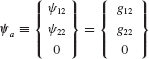
Example 17.1 For axial motion of the 3-DOF rod-mass system shown in Fig. 1, let the DOF sets be  ,
,  , and
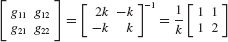
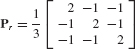
, and  . For a unit force applied to the left-hand mass (i.e., for faT = [0 1 0]): (a) Determine the attachment mode as defined by Eqs. 17.20 and 17.21. Sketch this mode. (b) Determine the self-equilibrated elastic load vector Pfa. (c) Determine the corresponding inertia-relief attachment mode as defined by Eqs. 17.31 and 17.32. Sketch this mode. The stiffness matrix and mass matrix for this system are, respectively,
Figure 1 A 3-DOF rod–mass system undergoing axial motion.


SOLUTION (a) From Eq. 17.21, the cantilever attachment mode corresponding to a unit force at DOF 2 is
where the cantilever flexibility matrix for the rod fixed at DOF 3 is
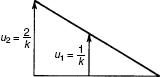
Therefore, the cantilever attachment mode is

which has the shape shown in Fig. 2.
Figure 2 Cantilever attachment mode.
(b) From Eq. 17.26, the inertia-relief projection matrix is

Equation 17.16 could be used to compute the rigid-body mode. However, for the present case, it is clear that the rigid-body mode consists of all masses displacing the same amount, so we can let

for which the generalized mass is
Therefore, the inertia-relief projection matrix is given by

or
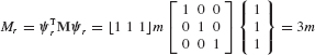
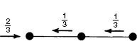
Therefore, the self-equilibrated force vector is

which is illustrated in Fig. 3.
Figure 3 Equilibrated force system.
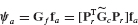
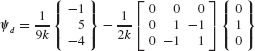
(c) From Eqs. 17.31 and 17.32 we get the following expression for the inertia-relief attachment mode corresponding to the force fa:
From Eqs. 2, 8, 9, 10, and 17.30, we get

Finally, the inertia-relief attachment mode corresponding to a unit force applied at the left-hand mass is

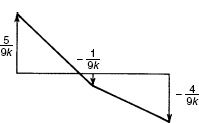
which has the shape shown in Fig. 4.
Figure 4 Inertia-relief attachment mode.
The reason for introducing inertia-relief attachment modes by using Eq. 17.31, rather than just using cantilever attachment modes as defined by Eq. 17.21, is the role played by Eq. 17.32 in the computation of residual flexibility, which is demonstrated in the next section.
17.4 FLEXIBILITY MATRICES AND RESIDUAL FLEXIBILITY
The complete set of component normal modes Φn and the corresponding set of eigenvalues Δnn are identified by the subscript n, whether these are the Ni fixed-interface modes, the Nf free-free flexible (flex) modes, or some other form of component normal modes.
Let the modal mass matrix and modal stiffness matrix for modes Φn be

respectively. Then the elastic flexibility matrix, G, of the component can be expressed in the following mode-superposition format:

This is a very important equation. Note that each column of the jth mode’s contribution to the elastic flexibility matrix has the shape of mode  . That is, the jth mode’s contribution to column i of G consists of the mode scaled by
  /Kj. For a free-free structure with Nf flexible modes, although the elastic flexibility matrix G of Eq. 17.34 and matrix Gf of Eq. 17.32 and illustrated in Fig. 17.6 are formed in different ways, they are numerically the same.
In this section we are concerned with components that have rigid-body freedom, in which case G is singular, with rank Nf. Regardless of whether the elastic flexibility matrix G is singular or not, from Eqs. 17.33b and 17.34 it can be shown that

Since model reduction is one of the major objectives in CMS, the normal mode set is usually reduced to a smaller set of kept normal modes, denoted by Φk, where Φn = [Φk Φd].2 The deleted normal modes, Φd, are generally all of the modes above some specified cutoff frequency. The portion of the flexibility matrix contributed by modes Φd is called the residual-flexibility matrix. It is given by

where G is the total flexibility matrix. Although it is not feasible to compute or measure all of the Φd modes, Eq. 17.36 is still very useful because Eq. 17.32 exists as an alternative to Eq. 17.34 for determining the elastic flexibility matrix G.
The matrix Gd will always be a singular matrix because of the modes deleted in Eq. 17.36. Also, because of the mass orthogonality and stiffness orthogonality of the kept modes to the deleted modes,

and because of the mass orthogonality between all rigid-body modes and all flexible-body modes,

Residual-flexibility attachment modes may be defined for forces applied at the interface coordinates, that is, for , by the following equation:
where Gf is given by Eq. 17.32. Thus, d contains the columns of the residual-flexibility matrix associated with the boundary DOFs.
Figure 17.7 shows the attachment mode shape for the component with a unit force at DOF7: The top figure includes all six flex modes, the middle figure is the contribution of two “kept” modes, and the bottom figure is the corresponding residual-flexibility attachment mode shape, that is, the difference between the top and middle figures. It is clear that the order of magnitude of the residual flexibility is smaller than that of the flexibility of the kept modes.
Figure 17.7 Illustration of residual flexibility.

Incorporation of d into the component mode set ensures complete representation of static deflection of the component due to forces applied at interface DOFs. In this sense it is closely related to the mode-acceleration method for incorporating static completeness in dynamic-response computations (Section 11.4). Hintz has given an extensive discussion of the need for statically complete component mode sets in Ref. [17.7]. We return to the topic of residual flexibility in Section 17.7.
Example 17.2 This example illustrates the use of Eq. 17.39 to determine a residual inertia-relief attachment mode for the three-mass system of Example 17.1, repeated in Fig. 1. (a) Determine the normal modes of the three-mass system of Example 17.1. (b) Let  ,
,  , and
, and  . Determine the residual inertia-relief attachment mode associated with a unit force applied to the left-hand mass. (c) Give a physical explanation of the result you obtained in part (b).
Figure 1 A 3-DOF rod–mass system undergoing axial motion.

SOLUTION (a) From Example 17.1 the algebraic eigenproblem can be written as

Then the frequencies are given by

or

This gives the characteristic equation

whose roots are

Mode shapes can be obtained from the top two equations of Eq. 1. Since the left end of the bar is DOF 2, let U2 = 1. Then the mode shapes are given by the following set of equations:

For mode 1, the rigid-body mode, ω12 = 0. So Eq. 5 becomes

Therefore, as expected, the rigid-body mode is given by

When normalized so that  , the normalized rigid-body mode is

For mode 2, ω22m = k. Therefore, Eq. 5 becomes

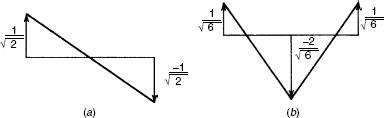
Thus, U1 = 0 and U3 = − 1, so mode 2 is the fundamental flexible mode, which has the form

When normalized so that  , the normalized mode
  is given by
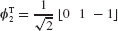
Finally, mode 3, normalized so that  can be shown to be

(Normally, “deleted modes” are not calculated. Mode 3 is calculated and shown here to help with the explanation in part c.) Modes 2 and 3 are shown in Fig. 2.
Figure 2 Flexible modes of a three-mass system: (a) mode ; (b) mode  .
.
(b) The residual inertia-relief attachment mode can be calculated from the following combination of Eqs. 17.32 and 17.39:

The first term on the right-hand side of Eq. 13 is the inertia-relief attachment mode that was determined in Eqs. 10 through 12 of Example 17.1. In the present problem, the kept flexible mode is mode 2, so

Hence,

From Example 17.1,

Finally, the residual inertia-relief attachment mode is
or

(c) As might have been expected, the residual attachment mode in the present case is exactly a multiple of , since it represents deformation of the three-mass system after removing rigid-body motion and after removing “kept” mode 2.
In determining the attachment mode, a unit force was placed at node 2 (left end). That applied force can be apportioned to the various modes as shown in Fig. 3. From Eqs. 15 and 16,
Figure 3 Modal contributions to an applied unit force.


This is exactly the deflection shape that would result from the application of the “mode 2 forces” in Fig. 3. Also, ψd, given by Eq. 18, is exactly the deflection shape produced by the “mode 3 forces.”
17.5 SUBSTRUCTURE COUPLING PROCEDURES
In this section, two versions of a generalized substructure coupling procedure for undamped structures are presented. Both procedures employ Lagrange multipliers to enforce component interface displacement compatibility equations (and other constraint equations, if applicable). The first coupling procedure applies to components that are assembled in the original physical-coordinate form. The second applies to coupling components after there has been a coordinate transformation to component generalized coordinates.
Let the system be composed of NS components, labeled  through
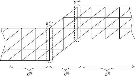
  . We consider here the case where the interface between any two adjacent components is represented by conforming discrete grid points, as illustrated in Fig. 17.8.3 Let these component interfaces be labeled
  through
  , where angle brackets, < · >, are used to label boundary segments.
Figure 17.8 Substructures and substructure interfaces.
Let ub be the set of all component interface coordinates of the assembled (i.e., coupled) system. Displacement compatibility along component interfaces can be enforced through specification of the connectivity matrices B(s) . Then

This implies that if  (p) and (q) are neighboring substructures, the portions of B(p) and B(q) that correspond to their shared boundary must be identical. This compatibility information can also be expressed in the form of interface displacement constraint equations, written in terms of physical displacement coordinates.
where the constraint matrix C and the merged vector of component physical coordinates have the following forms:

Since the interface displacement constraint equation in physical coordinates does not involve the interior coordinates ui(s), the substructure constraint matrices have the form

Two forms of system assembly will be useful in formulating specific substructure coupling methods: System Assembly in Physical Coordinates, employed in Section 17.7, and System Assembly in Generalized Coordinates, employed in Section 17.6 and again in Section 17.7.
17.5.1 System Assembly in Physical Coordinates
The synthesis of the system equation of motion is based on Lagrange’s equation of motion with Lagrange multipliers λ (see Section 8.5). The Lagrangian for the system of Ns coupled substructures can be written

where  is the system kinetic energy and
  is the system potential energy, given in terms of the physical coordinates by
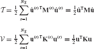
respectively. The block-diagonal uncoupled mass matrix M and the block-diagonal uncoupled stiffness matrix K are given by

Since the net work of the interconnecting boundary forces r within the coupled system is zero, the virtual work done on the system is given by
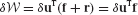
where, corresponding to Eq. 17.42b, the merged external force vector is
The system equations of motion can now be obtained by applying Lagrange’s equation in the form
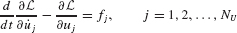
where uj refers to the jth element of the merged physical displacement vector u, and fj refers to the corresponding jth element of the vector of externally applied forces, f. Since they do not appear in the final expression for the virtual work, the mutually reactive interface constraint forces do not appear on the right-hand side of Eq. 17.49. Combining Eqs. 17.44, 17.45, and 17.47 with Eq. 17.49, we can write the NU equations of motion in the following matrix form:
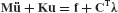
Comparing Eq. 17.50 with Eq. 17.1, we see that the term C(s)Tλ in Eq. 17.50 corresponds to the interface constraint force vector r(s) in Eq. 17.1. Since the substructure constraint matrices have the form given by Eq. 17.43, the actual interface constraint force acting on the boundary of component s is Cb(s)Tλ.
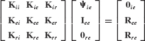
Since the NU displacement coordinates in Eq. 17.50 are not independent but are subject to the constraint equation, Eq. 17.41, we can combine these two equations to form the ( NU + NC ) set of hybrid coupled-system equations and write them in the following matrix form:
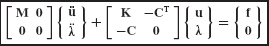
Application of Eq. 17.51 is illustrated in Section 17.7.
The following example illustrates for the three-component system in Fig. 17.8 the formation of the boundary displacement constraint equation and the physical meaning of the Lagrange multiplier vector.
Example 17.3 Treat the three components of the structure in Fig. 17.8 as superelements. That is, retain all original finite element DOFs, so that
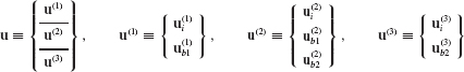
where the  and
and  boundary displacements of the substructures are identified by the subscripts b1 and b2, respectively (Fig. 1).
Figure 1 Interpretation of (a) substructure interface displacement compatibility, and (b) Lagrange multiplier interface constraint forces.

Let the interface displacement vector and the corresponding Lagrange multiplier vector have the forms

(a) Write the appropriate connectivity matrices as defined by Eq. 17.40. (b) Write the interface displacement constraint equation in the form prescribed by Eq. 17.41. (c) Form the CTλ term of Eq. 17.50, and use Fig. 1b to interpret the meaning of the λ vector.
SOLUTION (a) The connectivity matrices are defined by Eq. 17.40,

From Fig. 1a, Eq. 2a, and Eq. 3, the connectivity matrices are the boolean matrices (i.e., matrices of ones and zeros) in the following three equations:

(b) The same connectivity is expressed by the following interface displacement constraint equation:

Therefore, the interface displacement constraint matrix is

(c) Now we form CTλ using Eqs. 2b and 6:
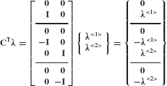
Therefore, λ<1> can be interpreted as the constraint force vector (tension positive) that enforces interface displacement compatibility at interface , and λ<2> is the constraint force vector (tension positive) that enforces interface displacement compatibility at interface , both illustrated in Fig. 1b.
17.5.2 System Assembly in Generalized Coordinates
Let us now formulate the system assembly process using the component generalized coordinates p. Displacement constraint equations such as Eqs. 17.41 and any other constraint equations that are to be imposed (say, NCp equations in all) can be written in terms of the  generalized coordinates p and combined to form a matrix constraint equation of the form

For example, if there are only two substructures, Eqs. 17.2 can be combined with the boundary displacement compatibility equation

to give the constraint equation

where ψb(s) refers to the boundary-coordinate partition of the component mode matrix ψ(s) of component s.
The synthesis of the system equation of motion can be based on Lagrange’s equation of motion with Lagrange multipliers, where the transformation to component generalized coordinates now precedes the assembly of components.[17.8, 17.12] With the vector of Lagrange multipliers now designated as σ, the Lagrangian for the system of Ns coupled substructures can be written

where is the system kinetic energy and is the system potential energy, given by

respectively. The block-diagonal uncoupled mass matrix Mp, the block-diagonal uncoupled stiffness matrix Kp, and the vector of component-mode coordinates p are given by

Since the net work of the interconnecting boundary forces r within the coupled system is zero, the virtual work done on the system is given by

where, corresponding to Eq. 17.57c, the transformed external force vector can be written in the following form:

The system equations of motion can now be obtained by applying Lagrange’s equation in the form

where pj refers to the jth element of the merged displacement vector p, and fpj refers to the corresponding jth element of the transformed vector of externally applied forces, fp. Since they do not appear in the final expression for the virtual work, the mutually reactive interface constraint forces do not appear on the right-hand side of Eq. 17.60. We can write the NP equations of motion in the following matrix form:

The term CpTσ in Eq. 17.61 corresponds to the interface constraint force vector, expressed in generalized coordinates.
Since the NP generalized coordinates in Eq. 17.61 are not independent but are subject to the constraint equation, Eq. 17.52, we can combine these two equations to form the NP + NCp set of coupled system equations in the following matrix form:

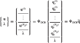
Many substructure coupling methods solve the coupled set of equations, Eq. 17.62, by introducing a linear transformation of the form[17.8, 17.12]

where q is the vector of independent system generalized coordinates. Let p be rearranged, if necessary, and partitioned into ND dependent coordinates pD and NP − ND linearly independent coordinates pI ≡ q, and let Eq. 17.52 be partitioned accordingly, giving

where CDD is a nonsingular square matrix. The coordinate transformation equation

defines both S and q. Then the vector of independent system generalized coordinates is q ≡ pI, and the substructure coupling matrix S is given by

Substitution of Eq. 17.63 into Eq. 17.61 and premultiplication of the resulting equation by ST gives
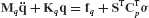
where

From Eqs. 17.64 and 17.66, it is seen that CPS = 0. Therefore, the system equation of motion, Eq. 17.67, becomes simply

Although Eq. 17.68 defines Mq, Kq, and fq in terms of matrix multiplication operations, the system matrices and force vector can usually be assembled from the substructure matrices by the “direct stiffness” assembly procedure, as illustrated in Section 17.6.
To summarize the generalized component-mode synthesis (CMS) procedure:
1. Choose the component modes to be included in each ψ(s). This defines the corresponding component generalized coordinates p(s).
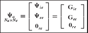
2. Using Eqs. 17.4a, b, and c, form all  .
.
3. Establish which of the coordinates in p will be the dependent coordinates, pD; the remainder form pI ≡ q.
4. Write the constraint equation (or equations) in the form of Eq. 17.54, and use Eq. 17.66 to solve for S.
5. Determine the coupled system matrices Mq and Kq using Eqs. 17.68a and b, respectively, and use Eq. 17.68c to determine the coupled system external force vector fq. These are the ingredients of Eq. 17.69, the final coupled system equation of motion.
The two substructure assembly procedures presented above describe a single level of substructuring, which is illustrated in Sections 17.6 and 17.7. Substructuring can also be employed to treat a structure that is partitioned into several levels of substructures, as discussed briefly in Section 17.8.
17.6 COMPONENT-MODE SYNTHESIS METHODS: FIXED-INTERFACE METHODS
Most applications of component-mode synthesis employ one of two approaches, which may be called fixed-interface-mode methods and free-interface-mode methods. The former employ fixed-interface normal modes and constraint modes, as illustrated in this section and in Section 17.8. The latter employ free-interface normal modes and attachment modes, as illustrated in Section 17.7. There are also some hybrid methods. It is possible to cite here only a sample of the significant papers dealing with the use of component modes in structural dynamics.
Although there had been previous applications of component modes, Hurty’s 1965 paper[17.2] provided the first comprehensive development of a finite-element-oriented CMS method based on constraint modes and fixed-interface modes. Craig and Bampton[17.4] simplified Hurty’s method by treating all interface degrees of freedom together rather than requiring the interface degrees of freedom to be separated into rigid-body freedoms and redundant interface freedoms. This method has been widely adopted because of its superior accuracy, its ease of implementation, and its efficient use of computer resources.
17.6.1 Fixed-Interface Displacement Transformation
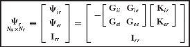
The displacement transformation of the Craig-Bampton Method employs a combination of fixed-interface normal modes (Eq. 17.7 and Fig. 17.3) and interface constraint modes (Eq. 17.13 and Fig. 17.5), and takes the form
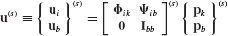
where the C-B transformation matrix is
where Φik is the interior partition of the matrix of kept fixed-interface modes and ψib is the interior partition of the constraint-mode matrix.
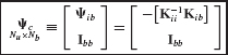
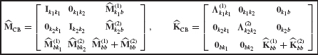
With component fixed-interface normal modes normalized according to Eq. 17.9, the reduced component mass and stiffness matrices, Eqs. 17.4, have the special forms

The zeros in the kb and bk partitions of  are the result of orthogonality equation 17.14. System Assembly in Generalized Coordinates, based on Eqs. 17.63 through 17.69, will now be used to assemble the Craig-Bampton reduced-order coupled-system mass and stiffness matrices.[17.4]
17.6.2 Craig–Bampton Method
The bottom row of Eq. 17.70 implies that

Therefore, in terms of component generalized coordinates, for a two-component system the interface compatibility equation, Eq. 17.53, becomes

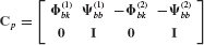
Equation 17.65 can be formed directly (see Problem 17.9 for application of Eqs. 17.64 and 17.66) and written in the form

so the component coupling matrix S is just the “direct-stiffness assembly” matrix. For a two-component system, component mass and stiffness matrices (Eq. 17.72) are assembled to form the following system reduced-order mass and stiffness matrices, respectively:
(An additional eigensolution can be performed on the bb partition in the lower right-hand corner of the  and
and  matrices, reducing the corresponding terms to Ibb and Λbb, respectively, and correspondingly modifying the kb and bk terms in .)
In summary, CMS models based on the use of fixed-interface modes plus interface constraint modes are essentially reduced-order superelements: All physical boundary coordinates are retained in Eq. 17.63 as independent generalized coordinates, greatly facilitating component coupling. Because of the simple, straightforward procedures for formulating the component modes employed by this method; because of the straightforward way in which components are coupled to form the component-mode system model; because of the sparsity patterns of the resulting system matrices and the ease of adding adding additional modal coordinates; and because this method also produces highly accurate models with relatively few component modes[17.9]; this method has been widely used and is available in a number of commercial finite element codes (e.g., MSC/NASTRAN[17.27]). Rixen[17.28] refers to this form of component assembly as primal assembly, as depicted in Fig. 17.1b.
The principal drawback of the CB method is that the system submatrices related to fixed-interface modes and constraint modes are difficult to verify experimentally. As presented above, all boundary coordinates are retained in the final Craig– Bampton reduced-order system model. For two-dimensional (i.e., plate and shell) structures, and particularly for three-dimensional solids, the number of interface DOFs can become very large. Farhat and Geradin [17.25] have presented an extension of the Craig–Bampton Method that permits coupling of substructures that have incompatible interface grids and have shown how to reduce the number of interface DOFs. Craig and Hale[17.23] have presented a variant of the Craig–Bampton Method that uses fixed-interface Krylov vectors instead of fixed-interface normal modes. Constraint modes and fixed-interface normal modes also form the basis for model reduction in the AMLS multilevel substructuring method, which is discussed briefly in Section 17.8.
Fransen[17.29] has compared the mode-displacement, mode-acceleration, and modal-truncation-augmentation methods for recovering the internal loads of Craig-Bampton reduced dynamic substructure models.
17.7 COMPONENT-MODE SYNTHESIS METHODS: FREE-INTERFACE METHODS
If a reduced set of component free-interface modes is used without including a complete set of either interface constraint modes or interface attachment modes, the component-mode set is not statically complete, as indicated in Section 17.4. This is true of the “classical” CMS method of using only a set of free-interface normal modes. The accuracy of reduced-order models produced by this method is unacceptable.[17.9] However, methods that employ free-interface normal modes together with attachment modes (including residual-flexibility attachment modes and/or inertia-relief attachment modes) have been used fairly widely, especially MacNeal’s Method[17.5] and Rubin’s Method[17.6], and have also been used in the context of experimental verification of finite element models.[17.17–17.19]
17.7.1 Augmented Free-Interface Displacement Transformation
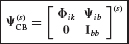
Let us assume that the typical component has rigid-body degrees of freedom. Then the basic displacement transformation for this class of free-interface methods employs a combination of rigid-body modes ψr (from Eq. 17.16), kept free-free normal modes Φk (from Eq. 17.11), and residual-flexibility attachment modes ψd (from Eq. 17.39). To simplify the following discussion, the rigid-body modes can be written in the following two-partition form:
These rigid-body modes are then combined with the kept free-interface flexible modes and with residual-flexibility attachment modes to give the following coordinate transformation:

As noted in Section 17.1, if a load is prescribed at an “interior” DOF, this DOF is relabeled as a “boundary” DOF. From Eq. 17.78, the augmented free-interface transformation matrix is4
(Note: As in Eq. 17.39, the columns of the residual-flexibility attachment mode matrix ψd are labeled b, not d, because these modes are created by unit forces acting at the boundary degrees of freedom.)
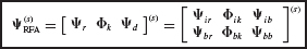
With mass-normalized rigid-body modes ψr and mass-normalized free-interface normal modes Φk, the component generalized mass matrix and stiffness matrix based on the free-interface transformation matrix are

where it can be shown that  . The zeros in these matrices are the result of orthogonality (e.g., Eqs. 17.37 and 17.38), and the residual flexibility term ψbb of
  is due to Eq. 17.35. The formulation above is a consistent Ritz transformation; residual-flexibility effects are included in both the stiffness and mass matrices.
17.7.2 Craig–Chang Method
A free-interface method that employs the RFA component modes in Eqs. 17.79 and 17.80 was introduced in Refs.[17.8] and [17.12]. This free-interface method has been referred to in the literature as the Craig-Chang Method. Due to the zeros in the third row of the RFA mass matrix and stiffness matrix in Eq. 17.80, the component equation of motion for pd becomes
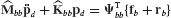
where the boundary force term comes from Eq. 17.5. Two assumptions are made: (1) that the inertia term can be neglected and a pseudostatic solution obtained for the residual-flexibility coordinates, pd, and (2) that the interface reaction forces alone drive the behavior of the residual-flexibility coordinates, as is the case for free vibration. Then since  Eq. 17.81 reduces to

Since ψbb is nonsingular,

When two components are coupled, the interface reaction forces acting on the two components satisfy the following force constraint equation:

This can be used as an additional equation of constraint, as demonstrated in the following example.
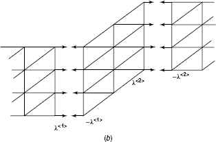
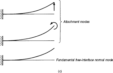
Example 17.4 Let each of the two beam components in Fig. 1a be represented by a set of free-interface normal modes and a set of residual-flexibility attachment modes defined by forces applied at the interface (boundary) coordinates. Figure 1c illustrates the forces applied to component (1) to define its attachment modes and also illustrates one free-interface normal mode.
Figure 1 Component-mode synthesis: (a) coupled beam system; (b) cantilever beam components; (c) component modes.

Figure 1 (continued)
Let the displacement transformation for each component have the form
Let the unassembled component generalized coordinate vector have the form

and let the final system generalized coordinate vector have the form

Determine the constraint matrix Cp of Eq. 17.52 that corresponds to the displacement constraint of Eq. 17.53 and the force constraint of Eq. 17.84.
SOLUTION The two equations of constraint to be enforced are, from Eq. 17.53,

and from Eqs. 17.83 and 17.84,

Finally, the constraint matrix has the form
where the top row corresponds to the displacement constraint of Eq. 4 and the bottom row corresponds to the force constraint of Eq. 5.
It is left as Problem 17.11 for the transformation matrix S of Eqs. 17.63 through 17.66 to be determined for a similar 2-component structure.
One advantage of this method is that all pd coordinates are reduced out, leaving only the kept free-interface modal coordinates in the final system model. However, it is typical of free-interface methods that the final reduced-order coupled system mass and stiffness matrices lose the sparsity exhibited by the RFA component matrices of Eqs. 17.80. That is the case for this free-interface method. One free-interface method that does preserve the sparsity of Eqs. 17.80 in the assembled reduced-order model is a method that Rixen developed recently and named the Dual Craig–Bampton Method.[17.28]
17.7.3 Rixen’s Dual C-B Method
As noted immediately following Eq. 17.50 and illustrated in Example 17.3, the Lagrange multiplier vector λ contains the interface forces that enforce the NC interface displacement constraints, Eq. 17.41. Therefore, the displacement transformation proposed by Rixen has the form

Note how this equation differs from the expression for u(s) in Eq. 17.78, which does not require that the residual flexibility generalized coordinates pd(s) be identified with the constraint forces.
Starting with Eq. 17.51, repeated here,
we use Eq. 17.85a and approximate the vector of unknowns as
where the Dual C-B transformation matrix has the form

Blank blocks of the transformation matrix are all zeros; dots indicate that the diagonal blocks and right-hand-column blocks follow the indicated patterns.
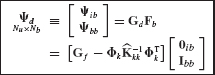
Combining Eqs. 17.51 and 17.86 in “Rayleigh–Ritz fashion,” we get the following reduced-order hybrid system equation of motion5:

Where

The reduced-order hybrid system mass matrix  is block diagonal, and the reduced-order hybrid system stiffness matrix
  is block diagonal except for additional terms in the λ row and λ column.[17.28] Therefore, this Dual Craig-Bampton formulation preserves sparsity of the final mass and stiffness matrices. Whereas the coupling in the Craig-Bampton formulation is in the mass matrix (Eq. 17.76), the coupling terms in the Dual Craig-Bampton formulation are in the stiffness matrix.
This method does not employ a true Rayleigh-Ritz transformation of displacement coordinates, but transforms the hybrid coupled-system equations with a hybrid transformation matrix. Therefore, the eigenvalues of the reduced-order model are not guaranteed to be upper bounds and can even be negative. However, on fairly large sample problems, the method is reported to have produced excellent results.[17.28]
17.8 BRIEF INTRODUCTION TO MULTILEVEL SUBSTRUCTURING
Recently, Bennighof6 and his graduate assistants have developed an automated multilevel substructuring algorithm called the AMLS Method.[17.20,17.21,17.30] This method uses an automated partitioning procedure that creates many levels of substructures (up to 30 or more levels) for finite element models having up to several million degrees of freedom. Then, using constraint modes and fixed-interface normal modes, in a manner similar to that discussed in Section 17.6.1, AMLS efficiently produces reduced-order models for which it calculates accurate eigensolutions and frequency-response solutions.
The development of AMLS was motivated by the need to compute frequency response, over a broad frequency range, of structures modeled with several million degrees of freedom. Direct computation of solutions of the FE model’s frequency-response equations at hundreds of frequencies for models that large is prohibitive, so mode superposition has traditionally been used instead. With the modal frequency-response approach, the computational burden is shifted to solving for thousands of modes of million-DOF models. However, use of the Block Lanczos Algorithm to perform these eigensolutions requires so much data bandwidth that only vector supercomputers are capable of performing large-scale frequency-response analyses with reasonable job turnaround. With AMLS, memory requirements for substructure eigen-problems are much smaller than for the global FE eigenvalue problem. Truncation of the substructure eigensolutions defines the subspace that is used for approximating the global eigensolution needed for modal frequency-response analysis. The accuracy of the lowest-frequency approximate global eigenpairs is excellent, and the accuracy of the highest-frequency ones depends primarily on how severely the substructure eigensolutions are truncated. Consequently, AMLS enables the analyst to work with geometrically accurate FE models of complex structures generated directly from CAD representations and has made it possible for very large frequency-response problems to be solved using inexpensive computer workstation hardware rather than supercomputers.
This section, which was abstracted from Chapters 2 and 4 of Ref. 17.20, provides only a brief introduction to the concept of multilevel substructuring and indicates the significant computational benefits that have been demonstrated to date for this extension of component-mode synthesis. For further details, the reader should consult Refs.[17.20] and [17.21].
The AMLS algorithm consists of five phases:
1. Generate an FE model (e.g., use NASTRAN to generate K and M).
2. Reorder DOFs and partition K and M into substructures.
3. Transform matrices to create the reduced-order component-mode model.
4. Compute the reduced-order system eigensolution.
5. Compute the frequency-response solution.
17.8.1 Single-Level Substructuring
To point out several key differences between single- and multilevel substructuring, we begin with a rectangular plate divided into two components. In classic CMS literature, the plate in Fig. 17.9a would be said to consist of two components (or substructures) separated by a boundary. The reduced-order stiffness and mass matrices for the separate components would be generated and then assembled to form the reduced-order system model. By contrast, the AMLS implementation of multilevel substructuring starts in phase 1 with the fully assembled system stiffness and mass matrices for the plate and in phase 2 partitions them into three substructures: Subdomains 1 and 2 in Fig. 17.9a are labeled substructures 1 and 2, and the interface between subdomains 1 and 2 is also considered to be a substructure, labeled substructure 3. So the AMLS model is considered to have three substructures, whose DOFs correspond to the three displacement vectors x1, x2, and x3.
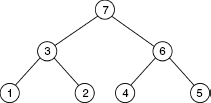
Figure 17.9 Rectangular plate partitioned into two subdomains (components): (a) plate divided into three substructures; (b) substructure tree diagram. (From [17.20].)
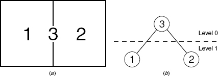
Figure 17.9b shows a graph of the simple relationship between the substructures. This graph is referred to as a substructure tree diagram and illustrates the relationships among the substructures pictured in Fig. 17.9a. Substructures 1 and 2 are referred to as the bottom-level substructures because there are no substructures below them on the diagram. Substructure 3 is a higher-level substructure and could also be called the parent of substructures 1 and 2. (In the present case, substructure 3 is also the highest-level substructure.) Substructure 3 is said to be at level 0; its children, substructures 1 and 2, are said to be at level 1. In typical applications of AMLS, there may be 30 or more such levels.
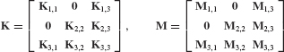
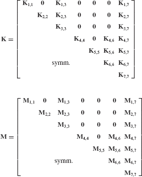
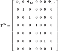
For the simple plate model in Fig. 17.9, the original assembled system stiffness and mass matrices would have the forms
From the AMLS perspective, the transformation of substructure 1 can be written

where Φ1 is the matrix of kept fixed-interface modes for substructure 1, and ψ1,3 is the constraint-mode matrix for constraint-mode shapes in the interior of substructure 1 due to unit displacements on the boundary DOFs that comprise substructure 3. That is, Φ1 contains the Nk1 lowest-frequency eigenvectors of the problem,

and the constraint modes are defined by the equation

The transformation of the second substructure can similarly be written

It should be noted that AMLS performs a final eigensolution on the interface DOFs, whereas the physical boundary coordinates would be retained in the classical Craig-Bampton single-level substructure method. This third substructure transformation is

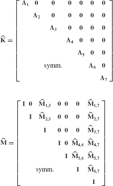
So the coordinate transformation of the entire model can be written

where the transformation matrix T has the formal structure
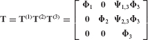
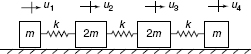
Finally, the reduced stiffness and mass matrices are given by

17.8.2 Multilevel Substructuring
The plate in Fig. 17.10 will now be used to introduce multilevel substructuring procedures, as implemented by AMLS. This will be referred to as the S4 model. Figure 17.11 illustrates a possible substructure numbering scheme for this S4 model, and Fig. 17.12 shows the corresponding substructure tree. For convenience, we introduce notation that refers to the sets of ancestors (e.g., “parent,” “grandparent”) and descendants (e.g., “child,” “grandchild”) of a substructure. Let  be defined as the set of all substructure indices j such that j is an ancestor of substructure i. And let
  be defined as the set of all substructure indices j such that j is a descendant of substructure i. Ancestors of a substructure are above it in the substructure tree; descendants are below it. From Fig. 17.11b and c it should become clear why in multilevel substructuring, boundaries
Figure 17.10 Plate partitioned into four subdomains (components). (From [17.20].)

Figure 17.11 Possible substructuring for the S4 model: (a) bottom-level substructures; (b) higher-level substructures; (c) highest-level substructure. (From [17.20].)
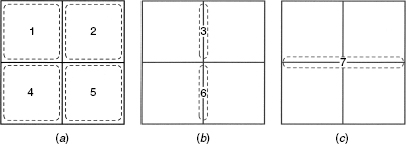
Figure 17.12 Substructure tree for the S4 model. (From [17.20].)
between substructures are also considered to be substructures. For example, although the substructure labeled 3 in Fig. 17.11b is on the boundary between substructures 1 and 2 (in Fig. 17.11a), it is the interior of the higher-level substructure whose boundary with substructure 6 is labeled substructure 7 in Fig. 17.11c.
It is important to note that in AMLS, all degrees of freedom at which external loads (including localized damping) can be applied are included in the highest-level substructure. In practice, substructures of approximately 1000 DOFs have been found to make phase 3 run efficiently.
For this problem, the stiffness and mass matrices may be partitioned as
Substructures are processed, starting with those on the lowest level and proceeding up the substructure tree. The interested reader can consult Ref. [17.20] for details. Here we just indicate the form of the coordinate transformation for the first substructure, the final coordinate transformation matrix, and the final reduced-order stiffness and mass matrices.
The coordinate transformation for the first substructure is
where, as before, Φ1 refers to the matrix of kept fixed-interface normal modes of substructure 1 and ψ1, j refers to a matrix of constraint modes over the interior of substructure 1 due to unit displacements on the boundary of substructure 1 that is designated as substructure j. Notice that the transformation matrix for substructure 1 deviates from the identity matrix only in blocks involving substructure 1 and its ancestors 3 and 7.
The final coordinate transformation is

All ηi’s except η7 are reduced sets of fixed-interface modal coordinates, but η7 must contain the full set of modal coordinates equal to the number of coordinates in x7 in order to preserve static completeness.
The final transformation matrix has the form

A column of this transformation matrix can be thought of as representing an admissible vector in a Rayleigh–Ritz formulation. For a bottom-level substructure (i.e., 1, 2, 4, and 5), these correspond simply to substructure eigenvectors. For a higher-level substructure, a column contains row entries for the substructure in question and row entries for all of that substructure’s descendants. The column for such a higher-level substructure may be called a multilevel extended eigenvector and is similar in concept to a constraint mode.
After the transformation at the highest level, the reduced-order system stiffness and mass matrices have the following forms:
If there are rigid-body modes of the structure, these will manifest themselves as zero eigenvalues of the highest-level substructure eigenproblem, here in Λ7.
Reference [17.20] discusses the complete multilevel computing strategy, including efficiencies that result from truncating the number of substructure eigenvectors (Eq. 4.7.3) and efficiencies that result when the number of output DOFs is small compared with the total number of finite element DOFs (Eq. 4.7.4).
17.8.3 Summary of an 8.4M-DOF Case Study
Reference 17.30 presents results obtained by using AMLS to compute an eigensolution for an 8.4M-DOF full vehicle (automobile) model. The frequency range of interest was 0 to 500 Hz, and the number of output DOFs was 245. Phase 2 of AMLS divided the 8.4M-DOF model automatically into 18,373 substructures on 31 levels. The substructure size ranged up to 2190 DOFs. For the given substructure eigenproblem cutoff frequency of 3750 Hz, phase 3 computed 135,924 substructure eigenvectors and projected the system K and M onto this eigenvector subspace. Phase 4 solved the reduced eigenproblem of order 135,924, looking for more than 11,000 eigenpairs. Finally, phase 5 computed the output at the 245 output DOFs. On a four-900-MHz-processor shared-memory computer having 8 GB of physical memory and 500 GB of disk space, the complete eigensolution for this 8.4M-DOF model took just over 6 hours, of which 3 hours was spent in phase 3 and 1 hours in phase 4.
REFERENCES
[17.1] W. C. Hurty, Dynamic Analysis of Structural Systems by Component Mode Synthesis, Technical Report 32-530, Jet Propulsion Laboratory, Pasadena, CA, January 1964.
[17.2] W. C. Hurty, “Dynamic Analysis of Structural Systems Using Component Modes,” AIAA Journal, Vol. 3, No. 4, 1965, pp. 678–685.
[17.3] R. M. Bamford, A Modal Combination Program for Dynamic Analysis of Structures (Revision No. 1), Technical Memorandum 33-290, Jet Propulsion Laboratory, Pasadena, CA, July 1, 1967.
[17.4] R. R. Craig, Jr. and M. C. C. Bampton, “Coupling of Substructures for Dynamic Analysis,” AIAA Journal, Vol. 6, No. 7, 1968, pp. 1313–1319.
[17.5] R. H. MacNeal, “A Hybrid Method of Component Mode Synthesis,” Journal of Computers & Structures, Vol. 1, No. 4, December 1971, pp. 581–601.
[17.6] S. Rubin, “Improved Component-Mode Representation for Structural Dynamic Analysis,” AIAA Journal, Vol. 13, No. 8, August 1975, pp. 995–1006.
[17.7] R. H. Hintz, “Analytical Methods in Component Modal Synthesis,” AIAA Journal, Vol. 13, No. 8, August 1975, pp. 1007–1016.
[17.8] R. R. Craig, Jr. and C.-J. Chang, “On the Use of Attachment Modes in Substructure Coupling for Dynamic Analysis,” Paper 77-045, presented at the AIAA/ASME 18th Structures, Structural Dynamics and Materials Conference, San Diego, CA, 1977.
[17.9] W. A. Benfield, C. S. Bodley, and G. Morosow, “Modal Synthesis Methods,” presented at the Space Shuttle Dynamics and Aeroelasticity Working Group Symposium on Substructure Testing and Synthesis, NASA-TM-X-72318, Marshall Space Flight Center, AL, 1972.
[17.10] R. R. Craig, Jr., “Coupling of Substructures for Dynamic Analysis: An Overview,” Paper AIAA-2000-1573, presented at the AIAA Dynamics Specialists Conference, Atlanta, GA, April 5–6, 2000.
[17.11] L. Meirovitch, Computational Methods in Structural Dynamics, Sijthoff & Noordhoff, Rockville, MD, 1980.
[17.12] R. R. Craig, Jr., Structural Dynamics: An Introduction to Computer Methods, Wiley, New York, 1981.
[17.13] N. M. M. Maia and J. M. M. Silva, eds., Theoretical and Experimental Modal Analysis, Research Studies Press, Baldock, Hertfordshire, England, and Wiley, New York, 1997.
[17.14] R. R. Craig, Jr. and Z. Ni, “Component Mode Synthesis for Model Order Reduction of Nonclassically Damped Systems,” AIAA Journal of Guidance, Control, and Dynamics, Vol. 12, No. 4, July–August 1989, pp. 577–584.
[17.15] J. A. Morgan, C. Pierre, and G. M. Hulbert, “Calculation of Component Mode Synthesis Matrices from Measured Frequency Response Functions, Part I: Theory,” Journal of Vibration and Acoustics, Vol. 120, No. 2, 1998, pp. 503–508.
[17.16] J. A. Morgan and R. R. Craig, Jr., “Comparison of Three Component Mode Synthesis Methods for Non-proportionally Damped Systems,” Paper AIAA-2000-1653, presented at the AIAA Dynamics Specialists Conference, Atlanta, GA, April 5–6, 2000.
[17.17] J. R. Admire, M. L. Tinker, and E. W. Ivey, “Mass-Additive Modal Test Method for Verification of Constrained Structural Models,” AIAA Journal, Vol. 31, No. 11, 1993, pp. 2148–2153.
[17.18] K. O. Chandler and M. L. Tinker, “A General Mass-Additive Method for Component Mode Synthesis,” Paper AIAA-97-1381, Proceedings of the 38th Structures, Structural Dynamics and Materials Conference, Kissimmee, FL, April 1997, pp. 93–103.
[17.19] M. L. Tinker, “Free-Suspension Residual Flexibility Testing of Space Station Pathfinder: Comparison to Fixed-Base Results,” presented at the 39th AIAA Structures, Structural Dynamics and Materials Conference, Long Beach, CA, April 1998.
[17.20] M. F. Kaplan, “Implementation of Automated Multilevel Substructuring for Frequency Response Analysis of Structures,” Ph.D. dissertation, The University of Texas at Austin, Austin, TX, December 2001.
[17.21] J. K. Bennighof and R. B. Lehoucq, “An Automated Multilevel Substructuring Method for Eigenspace Computation in Linear Elastodynamics,” SIAM Journal on Scientific Computing, Vol. 25, No. 6, 2004, pp. 2084–2106.
[17.22] C. Farhat and R. X. Roux, “A Method of Finite Element Tearing and Interconnecting and Its Parallel Solution Algorithm,” International Journal for Numerical Methods in Engineering, Vol. 32, 1991, pp. 1205–1227.
[17.23] R. R. Craig, Jr. and A. L. Hale, “Block–Krylov Component Synthesis Method for Structural Model Reduction,” AIAA Journal of Guidance, Control, and Dynamics, Vol. 11, No. 6, 1988, pp. 562–570.
[17.24] W. A. Benfield and R. F. Hruda, “Vibration Analysis of Structures by Component Mode Substitution,” AIAA Journal, Vol. 9, No. 7, July 1971, pp. 1255–1261.
[17.25] C. Farhat and M. Geradin, “On a Component Mode Synthesis Method and Its Application to Incompatible Substructures,” Computers & Structures, Vol. 51, 1994, pp. 459–473.
[17.26] C. Farhat, P.-S. Chen, and J. Mandel, “A Scalable Lagrange Multiplier Based Domain Decomposition Method for Time-Dependent Problems” International Journal for Numerical Methods in Engineering, Vol. 38, 1995, pp. 3831–3853.
[17.27] “Introduction to Superelements in Dynamic Analysis,” Chapter 10 in MSC/NASTRAN Reference Manual, Version 69, MacNeal–Schwendler Corporation, Los Angeles.
[17.28] D. J. Rixen, “A Dual Craig–Bampton Method for Dynamic Substructuring,” Journal of Computational Mathematics, Vol. 168, 2004, pp. 383–391.
[17.29] Fransen, S. H. J. A, “Data Recovery Methodologies for Reduced Dynamic Substructure Models with Internal Loads,” AIAA Journal, Vol. 42, No. 10, 2004, pp. 2130–2142.
[17.30] M. Kim, “An Efficient Eigensolution Method and Its Implementation for Large Structural Systems,” Ph.D. dissertation, The University of Texas at Austin, Austin, TX, May 2004.
PROBLEMS
The problems in this chapter employ simple axial-deformation components, and are intended to clarify the concepts and methods presented. Since several of the problems are linked together, the instructor should consider assigning all problems that are related to one another: for example, Problems 17.1, 17.2, and 17.9, or Problems 17.3, 17.8, and 17.10.
You may, if you wish use the computer (e.g., MAT-LAB) to solve any of the problems in this section. ISMIS can be used to set up the component matrices.
Problem Set 17.2
17.1 (a) Use Eq. 17.13 to determine the constraint mode for the axial-deformation component in Fig. P17.1,

where AE = constant, pA = constant, and

(b) Sketch this constraint mode.
17.2 (a) Letting u3 = 0, solve for the two fixed-interface modes of the axial-deformation component in Fig. P17.1. Normalize the modes so that M1 = M2 = ρAL. (b) Sketch these two normal modes.
Problem Set 17.3
17.3 Since the axial-deformation member in Fig. P17.1 is fixed at its left end, the equation that corresponds to Eq. 17.20 to define an attachment mode with unit force at DOF 3 would be

(a) Determine this attachment mode, ψa. (b) Sketch this attachment mode.
17.4 (a) Determine the three free-interface normal modes for the bar in Fig. P17.1. Scale the three modes so that M1 = M2 = M3 = ρAL. (b) Sketch these three normal modes. (c) Using the modal-expansion theorem of Eqs. 10.33 and 10.34, determine the coefficients c, in the expansion of the attachment mode determined in Problem 17.3 in terms of the free-interface modes determined in part (a). Note: This shows that the attachment mode is a linear combination of the three free-interface normal modes; it is not an independent vector.
17.5 (See Example 17.1.) For axial motion of the 3-DOF bar shown in Fig. P17.5, let the DOF sets be  ,
,  , and
, and  . AE = constant and ρA = constant. Use a consistent mass matrix for the bar. For a unit force applied to the left end of the bar (i.e., for
  ): (a) Determine the attachment mode as defined by Eqs. 17.20 and 17.21. Sketch this mode. (Note: The order of rows and columns of K are not the same here as in Eq. 17.20.) (b) Determine the self-equilibrated elastic load vector Pfa. (c) Determine the corresponding inertia-relief attachment mode as defined by Eqs. 17.31 and 17.32. Sketch this mode.

17.6 (See Example 17.1.) For axial motion of the 4-DOF free-free spring-mass system shown in Fig. P17.6, let the DOF sets be  ,
,  , and
, and  . For a unit force applied to the left-hand mass (i.e., for
  ): (a) Determine the attachment mode as defined by Eqs. 17.20 and 17.21. Sketch this mode. (Note: The order of rows and columns of K are not the same here as in Eq. 17.20.) (b) Determine the self-equilibrated elastic load vector Pfa. (c) Determine the corresponding inertia-relief attachment mode as defined by Eqs. 17.31 and 17.32. Sketch this mode.
Problem Set 17.4
17.7 (See Example 17.2.) For axial motion of the 4-DOF free-free spring-mass system shown in Fig. P17.6, let the DOF sets be , , and . (a) Determine the four free-interface normal modes for the spring-mass system in Fig. P17.6. Normalize the modes so that M1 = M2 = M3 = M4 = m. (b) Sketch these four normal modes. (c) Let  ,
,  , and
, and  . Determine the residual inertia-relief attachment mode, corresponding to Eq. 17.39, associated with a unit force applied to the left-hand mass (i.e., for ). Sketch this mode.
17.8 (a) Determine the three free-interface normal modes for the cantilever bar in Fig. P17.1. Normalize the modes so that M1 = M2 = M3 = ρAL. (b) Sketch these three normal modes. (c) Let  Determine the residual flexibility matrix, corresponding to Eq. 17.36. (d) Determine the residual flexibility attachment mode, corresponding to Eq. 17.39, for a unit force applied to the right end of the bar in Fig. P17.1 (i.e., for
  ). Sketch this mode.
Problem Set 17.6
17.9 In Eq. 17.75 the coupling matrix S that relates the p component-mode coordinates and the q system coordinates is formed “directly,” where, for a two-component system, these vectors have the following forms given in Eq. 17.75:

(a) Write the displacement constraint matrix Cp in the format given in Eq. 17.64, letting pb(1) ≡ ub be the independent boundary DOF and pb(2) be the dependent boundary coordinate. Let pk1(1) ≡ qb1(1) and pk2(2) ≡ qk2(2) be independent fixed-interface modal coordinates. (b) Using Eq. 17.66, form the coupling transformation matrix S.
17.10 For each of the two components in Fig. P17.10, use the component modes determined in Problems 17.1 and 17.2 to construct a Craig–Bampton system model like the one described in Sections 17.6.1 and 17.6.2 as follows: (a) Use Eqs. 17.72 to form  keeping only the lowest-frequency fixed-interface normal mode for each component. (b) Use Eq. 17.76a to form the system mass matrix, . (c) Use Eq. 17.76b to form the system stiffness matrix, . (d) Solve the 3-DOF system eigenproblem in Craig-Bampton format.

Problem Set 17.7
17.11 For each of the two components in Fig. P17.10, use the answers from Problem 17.8 to construct a Craig–Chang type of system model like the one described in Section 17.7.2. Keep one free-interface normal mode and one residual-flexibility attachment mode for each component. To correspond with the order of coordinates in Eqs. 17.63 through 17.68, let
(a) Form the connectivity matrix Cp as in Example 17.4, but with the p coordinates rearranged as in Eq. 1. The first row of the matrix should be the interface displacement constraint, and the second row should be the interface reaction-force constraint. (See Example 17.4 for an example of the constraint matrix for a similar coupled-beam problem.) (b) Following Eqs. 17.64 through 17.66, solve for the substructure coupling matrix S corresponding to the constraint matrix that you set up in part (a). (c) Form the component generalized mass matrices:  (d) Assemble the uncoupled mass matrix Mp and the uncoupled stiffness matrix Kp, using terms from the component matrices formed in part (c), but inserting them according to the order of the p coordinates in Eq. 1. (e) Using the results of parts (b) and (d), and using Eqs. 17.68a and b, form the coupled-system mass matrix Mq and Kq, respectively. These constitute the 2-DOF reduced-order Craig-Chang model. (f) Use the mass matrix and stiffness matrix from part (e) to solve for the two eigenvalues.
17.12 For each of the two components in Fig. P17.10, use the answers from Problem 17.8 to construct a Dual C-B system model like the one described in Section 17.7.3 as follows: (a) Form the connectivity matrices C(1) and C(2) that enforce compatibility of the component tip displacements u3(1) and u3(2) by writing the interface displacement constraint equation as in part (b) of Example 17.3. (Note: There is only one constraint equation at the one interface between the two components. Correspondingly, there is only one Lagrange multiplier for this problem.) (b) Using the kept free-interface normal mode and the residual flexibility matrix from part (c) of Problem 17.8 and the constraint matrices from part (a) above, form the Dual C-B Transformation matrix ΨDCB, as given in Eq. 17.87. (Note: Since both components of the coupled system have one fixed end, there will be no submatrices corresponding to rigid-body modes.) (d) Use Eqs. 17.89a and b to form the complete 3-DOF reduced-order hybrid system matrices and respectively. (e) Solve the 3-DOF Dual C-B system eigenproblem.
1This flexibility matrix is also called a pseudoinverseof the (singular) system stiffness matrix and is symbolized by  .
.
2Rigid-body modes, if there are any, are not included in the normal mode sets  .
.
3References [17.25] and [17.26] generalize the procedure discussed here to nonconforming interfaces.
4The subscript RFA signifies rigid-body modes plus free-interface modes plus attachment modes.
5Note that the constraint is applied directly in physical coordinates and that the transformation to component generalized coordinates includes the Lagrange multiplier vector and well as the component displacement coordinate vector. Therefore, this is not strictly a Rayleigh–Ritz transformation.
6Professor Jeffrey K. Bennighof, <jkb@vibes.ae.utexas.edu>.