Detection of stationarity

There are multiple methods that can help us in figuring out whether the data is stationary, listed as follows:

• Plotting the data: Having a plot of the data with respect to the time variable can help us to see whether it has got a trend. We know from the definition of stationarity that a trend in the data means that there is no constant mean and variance. Let's do this in Python. For this example, we are using international airline passenger data.

First, let's load all the required libraries, as follows:

 from pandas import Series
from matplotlib import pyplot
%matplotlib inline

data = Series.from_csv('AirPassengers.csv', header=0)
  series.plot()
  pyplot.show()

We will get the following output:

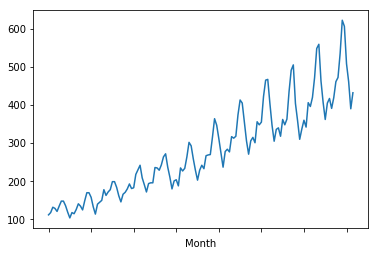
It is quite clear from the plot that there is an increasing trend here and that it would vindicate our hypothesis that it is a non-stationary series.

• Dividing the data set and computing the summary: The next method would be to divide the data series into two parts and compute the mean and variance. By doing this, we will be able to figure out whether the mean and variance are constant. Let's do this by using the following code:

X = data.values
partition =int(len(X) / 2)
X1, X2 = X[0:partition], X[partition:]
mean1, mean2 =np.nanmean(X1),np.nanmean(X2)
var1, var2 = np.nanvar(X1), np.nanvar(X2)
print('mean1=%f, mean2=%f' % (mean1, mean2))
print('variance1=%f, variance2=%f' % (var1, var2))

The output is as follows:

mean1=182.902778, mean2=377.694444 variance1=2244.087770, variance2=7367.962191

We can see that the mean and variance of series 1 and series 2 are not equal, and so we can conclude that the series is not stationary.

• Augmented Dickey-Fuller test: The augmented Dickey-Fuller test is a statistical test that tends to give an indication with a certain level of confidence as to whether the series is stationary. A statistical test takes the data and tests our hypothesis about the data using its assumption and process. Eventually, it yields the result with a certain degree of confidence, which helps us in taking the decision.

This test is nothing but the unit root test, which tries to find out whether the time series is influenced by the trend. It makes use of the autoregressive (AR) model and optimizes the information criterion at different lag values.

Here, the null hypothesis is as follows:

• H_o: The time series has got the unit root, which implies that the series is nonstationary

The alternate hypothesis is as follows:

• H₁: The time series doesn't have a unit root and, as such, it is stationary

As we know from the rules of hypothesis testing, if we have chosen a significance level of 5% for the test, then the result would be interpreted as follows:

If p-value >0.05 =>, then we fail to reject the null hypothesis. That is, the series is nonstationary.

If p-value <0.05 =>, then the null hypothesis is rejected which means that the series is stationary.

Let's perform this in Python:

1. First, we will load the libraries, as follows:

import pandas as pd
import numpy as np
import matplotlib.pylab as plt
%matplotlib inline
from matplotlib.pylab import rcParams
rcParams['figure.figsize'] = 25, 6

2. Next, we load the data and time plot as follows:

data = pd.read_csv('AirPassengers.csv')
print(data.head())
print('\n Data Types:')
print(data.dtypes)

The output can be seen in the following diagram:

3. We then parse the data as follows:

dateparse = lambda dates: pd.datetime.strptime(dates, '%Y-%m')
data = pd.read_csv('./data/AirPassengers.csv', parse_dates=['Month'], index_col='Month',date_parser=dateparse)
print(data.head())

We then get the following output:

ts= data["#Passengers"]
ts.head()

From this, we get the following output:

4. Then we plot the graph, as follows:

plt.plot(ts)

The output can be seen as follows:

5. Let's create a function to perform a stationarity test using the following code:

from statsmodels.tsa.stattools import adfuller
def stationarity_test(timeseries):
 dftest = adfuller(timeseries, autolag='AIC')
 dfoutput = pd.Series(dftest[0:4], index=['Test Statistic','p-value','#Lags Used','Number of Observations Used'])
 for key,value in dftest[4].items():
               dfoutput['Critical Value (%s)'%key] = value
 print(dfoutput)

stationarity_test(ts)

The output can be seen as follows:

Since p-value > 0.05 and the t-statistic is greater than all the critical values (1%,5%,10%), tt implies that the series is nonstationary as we failed to reject the null hypothesis.

So what can be done if the data is nonstationary? We use differencing to make the nonstationary data into stationary data.