The data that is given in this case study is about patients who were detected with two kinds of breast cancer:
- Malignant
- Benign
A number of features are given here that have characteristics in regard to the cell nuclei that have been computed from the fine-needle aspiration (FNA) of a breast mass. Based on these features, we need to predict whether the cancer is malignant or benign. Follow these steps to get started:
- Import all the required libraries:
import numpy as np
import pandas as pd
import seaborn as sns
import matplotlib.pyplot as plt
%matplotlib inline
from sklearn import preprocessing
from sklearn.model_selection import train_test_split
from sklearn.metrics import confusion_matrix
#importing our parameter tuning dependencies
from sklearn.model_selection import (cross_val_score, GridSearchCV,StratifiedKFold, ShuffleSplit )
#importing our dependencies for Feature Selection
from sklearn.feature_selection import (SelectKBest, RFE, RFECV)
from sklearn.ensemble import ExtraTreesClassifier
from sklearn.cross_validation import ShuffleSplit
from sklearn.ensemble import RandomForestClassifier
from sklearn.metrics import f1_score
from collections import defaultdict
# Importing our sklearn dependencies for the modeling
from sklearn.ensemble import RandomForestClassifier
from sklearn.preprocessing import StandardScaler
from sklearn.cross_validation import KFold
from sklearn import metrics
from sklearn.metrics import (accuracy_score, confusion_matrix,
 classification_report, roc_curve, auc)
- Load the breast cancer data:
data= pd.read_csv("breastcancer.csv")
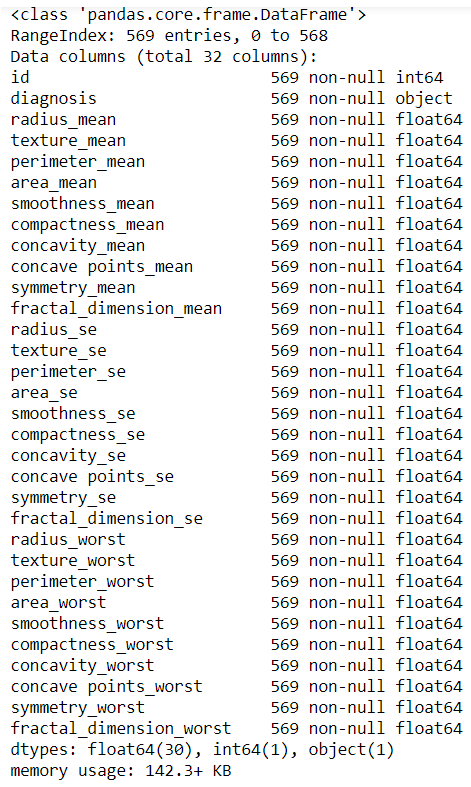
- Let's understand the data:
data.info()
We get the following output:
- Let's consider data.head() here:
data.head()
From this, we get the following output:

- We get the data diagnosis from the following code:
data.diagnosis.unique()
The following is the output for the preceding code:

- The data is described as follows:
data.describe()
We get this output from the preceding code:

data['diagnosis'] = data['diagnosis'].map({'M':1,'B':0})

datas = pd.DataFrame(preprocessing.scale(data.iloc[:,1:32]))
datas.columns = list(data.iloc[:,1:32].columns)
datas['diagnosis'] = data['diagnosis']

datas.diagnosis.value_counts().plot(kind='bar', alpha = 0.5, facecolor = 'b', figsize=(12,6))
plt.title("Diagnosis (M=1, B=0)", fontsize = '18')
plt.ylabel("Total Number of Patients")
plt.grid(b=True)

data_mean = data[['diagnosis','radius_mean','texture_mean','perimeter_mean','area_mean','smoothness_mean', 'compactness_mean', 'concavity_mean','concave points_mean', 'symmetry_mean', 'fractal_dimension_mean']]

plt.figure(figsize=(10,10))
foo = sns.heatmap(data_mean.corr(), vmax=1, square=True, annot=True)

from sklearn.model_selection import train_test_split, cross_val_score, cross_val_predict
from sklearn import metrics
predictors = data_mean.columns[2:11]
target = "diagnosis"
X = data_mean.loc[:,predictors]
y = np.ravel(data.loc[:,[target]])
# Split the dataset in train and test:
X_train, X_test, y_train, y_test = train_test_split(X, y, test_size=0.2, random_state=0)
print ('Shape of training set : %i & Shape of test set : %i' % (X_train.shape[0],X_test.shape[0]) )
print ('There are very few data points so 10-fold cross validation should give us a better estimate')
The preceding input gives us the following output:

param_grid = {
 'n_estimators': [ 25, 50, 100, 150, 300, 500],
 "max_depth": [ 5, 8, 15, 25],
 "max_features": ['auto', 'sqrt', 'log2']
 }
#use OOB samples ("oob_score= True") to estimate the generalization accuracy.
rfc = RandomForestClassifier(bootstrap= True, n_jobs= 1, oob_score= True)
#let's use cv=10 in the GridSearchCV call
#performance estimation
#initiate the grid
grid = GridSearchCV(rfc, param_grid = param_grid, cv=10, scoring ='accuracy')
#fit your data before you can get the best parameter combination.
grid.fit(X,y)
grid.cv_results_

# Let's find out the best scores, parameter and the estimator from the gridsearchCV
print("GridSearhCV best model:\n ")
print('The best score: ', grid.best_score_)
print('The best parameter:', grid.best_params_)
print('The best model estimator:', grid.best_estimator_)
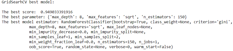
# model = RandomForestClassifier() with optimal values
model = RandomForestClassifier(bootstrap=True, class_weight=None, criterion='gini',
 max_depth=8, max_features='sqrt', max_leaf_nodes=None,
 min_impurity_decrease=0.0, min_impurity_split=None,
 min_samples_leaf=1, min_samples_split=2,
 min_weight_fraction_leaf=0.0, n_estimators=150, n_jobs=1,
 oob_score=True, random_state=None, verbose=0, warm_start=False)
model.fit(X_train, y_train)

print("Performance Accuracy on the Testing data:", round(model.score(X_test, y_test) *100))
From this, we can see that the performance accuracy on the testing data is 95.0:
#Getting the predictions for X
y_pred = model.predict(X_test)
print('Total Predictions {}'.format(len(y_pred)))
Here, the total predictions is 114:
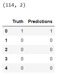
truth = pd.DataFrame(y_test, columns= ['Truth'])
predictions = pd.DataFrame(y_pred, columns= ['Predictions'])
frames = [truth, predictions]
_result = pd.concat(frames, axis=1)
print(_result.shape)
_result.head()
# 10 fold cross-validation with a Tree classifier on the training dataset# 10 fold
#splitting the data, fitting a model and computing the score 10 consecutive times
cv_scores = []
scores = cross_val_score(rfc, X_train, y_train, cv=10, scoring='accuracy')
cv_scores.append(scores.mean())
cv_scores.append(scores.std())

#cross validation mean score
print("10 k-fold cross validation mean score: ", scores.mean() *100)
From this, we can see that the 10 k-fold cross validation mean score is 94.9661835749:
# printing classification accuracy score rounded
print("Classification accuracy: ", round(accuracy_score(y_test, y_pred, normalize=True) * 100))
Here, we can see that the classification accuracy is 95.0:
# Making the Confusion Matrix
cm = confusion_matrix(y_test, y_pred)
plt.figure(figsize=(12,6))
ax = plt.axes()
ax.set_title('Confusion Matrix for both classes\n', size=21)
sns.heatmap(cm, cmap= 'plasma',annot=True, fmt='g') # cmap
plt.show()

# The classification Report
target_names = ['Benign [Class 0]', 'Malignant[Class 1]']
print(classification_report(y_test, y_pred, target_names=target_names))

y_pred_proba = model.predict_proba(X_test)[::,1]
fpr, tpr, _ = metrics.roc_curve(y_test, y_pred_proba)
auc = metrics.roc_auc_score(y_test, y_pred_proba)
plt.plot(fpr,tpr,label="curve, auc="+str(auc))
plt.legend(loc=4)
plt.show()

The preceding graph is a receiver operating characteristic (ROC) metric, which is used to evaluate classifier output quality using cross-validation.
The preceding plot shows the ROC response to our chosen features (['compactness_mean', 'perimeter_mean', 'radius_mean', 'texture_mean', 'concavity_mean', 'smoothness_mean']) and the diagnosis-dependent variable that was created from k-fold cross-validation.
A ROC area of 0.99 is quite good.