The Kernel PCA is an algorithm that not only keeps the main spirit of PCA as it is, but goes a step further to make use of the kernel trick so that it is operational for non-linear data:
- Let's define the covariance matrix of the data in the feature space, which is the product of the mapping function and the transpose of the mapping function:

It is similar to the one we used for PCA.
- The next step is to solve the following equation so that we can compute principal components:

Here, CF is the covariance matrix of the data in feature space, v is the eigenvector, and λ (lambda) is the eigenvalues.
- Let's put the value of step 1 into step 2 – that is, the value of CF in the equation of step 2. The eigenvector will be as follows:

Here,  is a scalar number.
- Now, let's add the kernel function into the equation. Let's multiply Φ(xk) on both sides of the formula,
 :
:

- Let's put the value of v from the equation in step 3 into the equation of step 4, as follows:

- Now, we call K
 . Upon simplifying the equation from step 5 by keying in the value of K, we get the following:

On doing eigen decomposition, we get the following:

On normalizing the feature space for centering, we get the following result:

Now, let's execute the Kernel PCA in Python. We will keep this simple and work on the Iris dataset. We will also see how we can utilize the new compressed dimension in the model:
- Let's load the libraries:
import numpy as np # linear algebra
import pandas as pd # data processing
import matplotlib.pyplot as plt
from sklearn import datasets
- Then, load the data and create separate objects for the explanatory and target variables:
iris = datasets.load_iris()
X = iris.data
y = iris.target
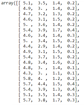
- Let's have a look at the explanatory data:
X
- Let's split the data into train and test sets, as follows:
from sklearn.model_selection import train_test_split
X_train, X_test, y_train, y_test = train_test_split(X, y, test_size = 0.25, random_state = 0)
- Now, we can standardize the data:
from sklearn.preprocessing import StandardScaler
sc = StandardScaler()
X_train = sc.fit_transform(X_train)
X_test = sc.transform(X_test)
- Let's have a look at X_train:
X_train
The output is as follows:

- Now, let's apply the kernel PCA on this. Here, we are trying to condense the data into just two components. The kernel that's been chosen here is the radial basis function:
from sklearn.decomposition import KernelPCA
kpca = KernelPCA(n_components = 2, kernel = 'rbf')
X_train2 = kpca.fit_transform(X_train)
X_test2 = kpca.transform(X_test)
We have got the new train and test data with the help of the kernel PCA.
- Let's see what the data looks like:
X_train2
We get the following as output:

Now, we've got two components here. Earlier, X_train showed us four variables. Now, the data has been shrunk into two fields.