Now we are ready to understand SVMs. SVM is an algorithm that enables us to make use of it for both classification and regression. Given a set of examples, it builds a model to assign a group of observations into one category and others into a second category. It is a non-probabilistic linear classifier. Training data being linearly separable is the key here. All the observations or training data are a representation of vectors that are mapped into a space and SVM tries to classify them by using a margin that has to be as wide as possible:
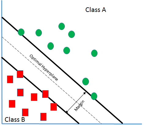
Let's say there are two classes A and B as in the preceding screenshot.
And from the preceding section, we have learned the following:
g(x) = w. x + b
Where:
- w: Weight vector that decides the orientation of the hyperplane
- b: Bias term that decides the position of the hyperplane in n-dimensional space by biasing it
The preceding equation is also called a linear discriminant function. If there is a vector x1 that lies on the positive side of the hyperplane, the equation becomes the following:
g(x1)= w.x1 +b >0
The equation will become the following:
g(x1)<0
If x1 lies on the positive side of the hyperplane.
What if g(x1)=0? Can you guess where x1 would be? Well, yes, it would be on the hyperplane, since our goal is to find out the class of the vector.
So, if g(x1)>0 => x1 belongs to Class A, g(x1)<0 => x1 belongs to Class B.
Here, it's evident that we can find out the classification by using the previous equation. But can you see the issue in it? Let's say the boundary line is like the following plot:

Even in the preceding scenario, we are able to classify those feature vectors here. But is it desirable? What can be seen here is that the boundary line or the classifier is close to the Class B. It implies that it brings in a large bias in the favor of Class A but penalizes Class B. As a result of that, due to any disturbances in the vectors close to the boundary, they might cross over and become part of Class A, which might not be correct. Hence, our goal is to find an optimal classifier that has got the widest margin, like what is shown in the following plot:
Through SVM, we are attempting to create a boundary or hyperplane such that the distance from each of the feature vectors to the boundary is maximized so that any slight noise or disturbance won't cause the change in classification. So, in this scenario, if we try to bring in certain yi which happens to be the class belonging to xi, we get the following:
yi= ± 1
yi (w.xi + b) will always be greater than 0. yi(w.xi + b) >0 because when xi ∈ class A, w.xi +b>0 then yi>0, so the whole term will be positive. Also, if xi ∈ class B, w.xi + b<0 then yi<0, and it will make the term positive.
So, now if we have to redesign it, we say the following:
w.xi + b> γ where γ is the measure of the distance of hyperplane from xi.
And if there is a hyperplane w.x + b = 0, then the distance of point x from the preceding hyperplane is as follows:
w.x + b/ ||w||
Hence, as mentioned previously:
w.x + b/ ||w|| ≥ γ
w.x + b ≥ γ.||w||
On performing proper scaling, we can say the following:
w.x + b ≥ 1 (since γ.||w|| = 1)
It implies that if there is a classification to be arrived at based on the previous result, it follows this:
w.x + b ≥ 1 if x ∈ class A and
w.x + b ≤ -1 if x ∈ class B
And now, again, if we bring in a class belonging to yi here, the equation becomes the following:
yi (w.xi + b) ≥ 1
But, if yi (w.xi + b) = 1, xi is a support vector. Next, we will learn what a support vector is.