There are different parameters to consider before applying gradient boosting for the breast cancer use case:
- Min_samples_split: The minimum number of samples required in a node to be considered for splitting is termed min_samples_split.
- Min_samples_leaf: The minimum number of samples required at the terminal or leaf node is termed min_samples_leaf.
- Max_depth: This is the maximum number of nodes allowed from the root to the farthest leaf of a tree. Deeper trees can model more complex relationships, however, causing the model to overfit.
- Max_leaf_nodes: The maximum number of nodes at the leaves in a tree. Since binary trees are created, a depth of n would produce a maximum of 2n leaves. Hence, either max_depth or max_leaf_nodes can be defined.
Now, we will apply gradient boosting for the breast cancer use case. Here, we are loading the libraries that are required to build the model:
from sklearn.ensemble import GradientBoostingClassifier
from sklearn.metrics import classification_report, confusion_matrix, roc_curve, auc
We are now done with the various steps of data cleaning and exploration while performing random forest. Now, we will jump right into building the model.
Here, we will perform a grid search to find out the optimal parameters for the gradient boosting algorithm:
param_grid = {
 'n_estimators': [ 25, 50, 100, 150, 300, 500], # the more parameters, the more computational expensive
 "max_depth": [ 5, 8, 15, 25],
 "max_features": ['auto', 'sqrt', 'log2']
 }
gbm = GradientBoostingClassifier(learning_rate=0.1,random_state=10,subsample=0.8)
#performance estimation
#initiate the grid
grid = GridSearchCV(gbm, param_grid = param_grid, cv=10, scoring ='accuracy')
#fit your data before you can get the best parameter combination.
grid.fit(X,y)
grid.cv_results_
We get the following output:

Now, let's find out the optimal parameters:
#Let's find out the best scores, parameter and the estimator from the gridsearchCV
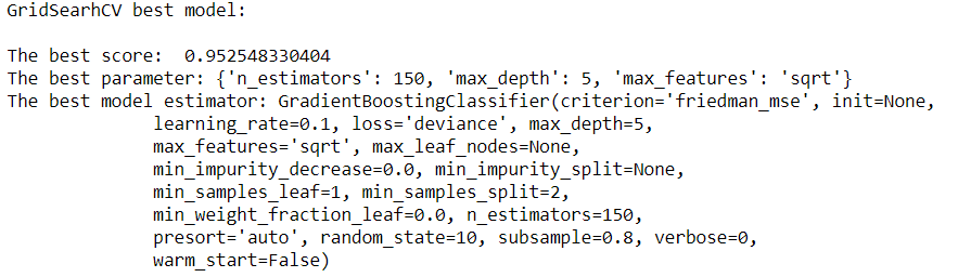
print("GridSearhCV best model:\n ")
print('The best score: ', grid.best_score_)
print('The best parameter:', grid.best_params_)
print('The best model estimator:', grid.best_estimator_)
The output can be seen as follows:
Now, we will build the model:
model2 = GradientBoostingClassifier(criterion='friedman_mse', init=None,
 learning_rate=0.1, loss='deviance', max_depth=5,
 max_features='sqrt', max_leaf_nodes=None,
 min_impurity_decrease=0.0, min_impurity_split=None,
 min_samples_leaf=1, min_samples_split=2,
 min_weight_fraction_leaf=0.0, n_estimators=150,
 presort='auto', random_state=10, subsample=0.8, verbose=0,
 warm_start=False)
model2.fit(X_train, y_train)

print("Performance Accuracy on the Testing data:", round(model2.score(X_test, y_test) *100))
The performance accuracy on the testing data is 96.0:
#getting the predictions for X
y_pred2 = model2.predict(X_test)
print('Total Predictions {}'.format(len(y_pred2)))
The total number of predictions is 114:
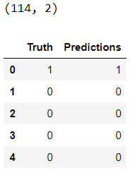
truth = pd.DataFrame(y_test, columns= ['Truth'])
predictions = pd.DataFrame(y_pred, columns= ['Predictions'])
frames = [truth, predictions]
_result = pd.concat(frames, axis=1)
print(_result.shape)
_result.head()
Let's perform cross-validation:
cv_scores = []

scores2 = cross_val_score(gbm, X_train, y_train, cv=10, scoring='accuracy')
cv_scores.append(scores2.mean())
cv_scores.append(scores2.std())

#cross validation mean score
print("10 k-fold cross validation mean score: ", scores2.mean() *100)
The 10 k-fold cross-validation mean score is 94.9420289855:
#printing classification accuracy score rounded
print("Classification accuracy: ", round(accuracy_score(y_test, y_pred2, normalize=True) * 100))
The classification accuracy is 96.0:
# Making the Confusion Matrix
cm = confusion_matrix(y_test, y_pred2)
plt.figure(figsize=(12,6))
ax = plt.axes()
ax.set_title('Confusion Matrix for both classes\n', size=21)
sns.heatmap(cm, cmap= 'plasma',annot=True, fmt='g') # cmap
plt.show()
By looking at the confusion matrix, we can see that this model is better than the previous one:
