SOM

Let's go through process of how SOMs learn:

1.  Each node's weights are initialized by small standardized random values. These act like coordinates for different output nodes.
2. The first row's input (taking the first row from all of the variables) is fed into the first node.
3. Now, we have got two vectors. If V is the current input vector and W is the node's weight vector, then we calculate the Euclidean distance, like so:

4. The node that has a weight vector closest to the input vector is tagged as the best-matching unit (BMU).
5. A similar operation is carried out for all the rows of input and weight vectors. BMUs are found for all.
6. Once the BMU has been determined for every iteration, the other nodes within the BMU's neighborhood are computed. Nodes within the same radius will have their weights updated. A green arrow indicates the radius. Slowly, the neighborhood will shrink to the size of just one node, as shown in the following diagram:

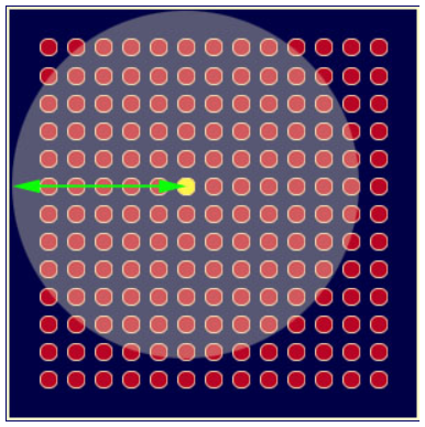
7. The most interesting part of the Kohonen algorithm is that the radius of the neighborhood keeps on shrinking. It takes place through the exponential decay function. The value of lambda is dependent on sigma. The number of iterations that have been chosen for the algorithm to run is given by the following equation:

8. The weights get updated via the following equation:

Here, this is as follows:

t= 1, 2... can be explained as follows:

• • L(t): Learning rate
  • D: Distance of a node from BMU
  • σ: Width of the function 

Now, let's carry out one use case of this in Python. We will try to detect fraud in a credit card dataset:

1. Let's load the libraries:

import numpy as np
import matplotlib.pyplot as plt
import pandas as pd

2. Now, it's time to load the data:

data = pd.read_csv('Credit_Card_Applications.csv')
X = data.iloc[:, :-1].values
y = data.iloc[:, -1].values

3. Next, we will standardize the data:

from sklearn.preprocessing import MinMaxScaler
sc = MinMaxScaler(feature_range = (0, 1))
X = sc.fit_transform(X)

4. Let's import the minisom library and key in the hyperparameters, that is, learning rate, sigma, length, and number of iterations:

from minisom import MiniSom
som = MiniSom(x = 10, y = 10, input_len = 15, sigma = 1.0, learning_rate = 0.5)
som.random_weights_init(X)
som.train_random(data = X, num_iteration = 100)    

5. Let's visualize the results:

from pylab import bone, pcolor, colorbar, plot, show
bone()
pcolor(som.distance_map().T)
colorbar()
markers = ['o', 's']
colors = ['r', 'g']
for i, x in enumerate(X):
 w = som.winner(x)
 plot(w[0] + 0.5,
 w[1] + 0.5,
 markers[y[i]],
 markeredgecolor = colors[y[i]],
 markerfacecolor = 'None',
 markersize = 10,
 markeredgewidth = 2)
show()

The following output will be generated from the preceding code:

We can see that the nodes that have a propensity toward fraud have got white backgrounds. This means that we can track down those customers with the help of those nodes:

mappings = som.win_map(X)
frauds = np.concatenate((mappings[(8,1)], mappings[(6,8)]), axis = 0)
frauds = sc.inverse_transform(frauds)                                         

 This will give you the pattern of frauds.