SVM example and parameter optimization through grid search

Here, we are taking a breast cancer dataset wherein we have classified according to whether the cancer is benign/malignant.

The following is for importing all the required libraries:

import pandas as pd
import numpy as np
from sklearn import svm, datasets
from sklearn.svm import SVC
import matplotlib.pyplot as plt
from sklearn.model_selection import train_test_split
from sklearn.model_selection import GridSearchCV
from sklearn.metrics import classification_report
from sklearn.utils import shuffle
%matplotlib inline

Now, let's load the breast cancer dataset:

BC_Data = datasets.load_breast_cancer()

The following allows us to check the details of the dataset:

print(BC_Data.DESCR)

This if for splitting the dataset into train and test:

X_train, X_test, y_train, y_test = train_test_split(BC_Data.data, BC_Data.target, random_state=0)

This is for setting the model with the linear kernel and finding out the accuracy:

C= 1.0
svm= SVC(kernel="linear",C=C)
svm.fit(X_train, y_train)
print('Accuracy-train dataset: {:.3f}'.format(svm.score(X_train,y_train)))
print('Accuracy- test dataset: {:.3f}'.format(svm.score(X_test,y_test)))

We get the accuracy output as shown:

Accuracy-train dataset: 0.967

Accuracy- test dataset: 0.958

Setting the model with the Gaussian/RBF kernel and accuracy is done like this:

svm= SVC(kernel="rbf",C=C)
svm.fit(X_train, y_train)
print('Accuracy-train dataset: {:.3f}'.format(svm.score(X_train,y_train)))
print('Accuracy- test dataset: {:.3f}'.format(svm.score(X_test,y_test)))

The output can be seen as follows:

Accuracy-train dataset: 1.000

Accuracy- test dataset: 0.629

It's quite apparent that the model is overfitted. So, we will go for normalization:

min_train = X_train.min(axis=0)
range_train = (X_train - min_train).max(axis=0)
X_train_scaled = (X_train - min_train)/range_train
X_test_scaled = (X_test - min_train)/range_train

This code is for setting up the model again:

svm= SVC(kernel="rbf",C=C)
svm.fit(X_train_scaled, y_train)
print('Accuracy-train dataset: {:.3f}'.format(svm.score(X_train_scaled,y_train)))
print('Accuracy test dataset: {:.3f}'.format(svm.score(X_test_scaled,y_test)))

The following shows the output:

Accuracy-train dataset: 0.948

Accuracy test dataset: 0.951

Now, the overfitting issue cannot be seen any more. Let's move on to having an optimal result:

parameters = [{'kernel': ['rbf'],
 'gamma': [1e-4, 1e-3, 0.01, 0.1, 0.2, 0.5],
 'C': [1, 10, 100, 1000]},
 {'kernel': ['linear'], 'C': [1, 10, 100, 1000]}]
clf = GridSearchCV(SVC(decision_function_shape='ovr'), parameters, cv=5)
clf.fit(X_train, y_train)
print("Best parameters set found on development set:")
print()
print(clf.best_params_)
print()
print("Grid scores on training set:")
print()
means = clf.cv_results_['mean_test_score']
stds = clf.cv_results_['std_test_score']
for mean, std, params in zip(means, stds, clf.cv_results_['params']):
 print("%0.3f (+/-%0.03f) for %r"
 % (mean, std * 2, params))
print()

With the help of grid search, we get the optimal combination for gamma, kernel, and C as shown:

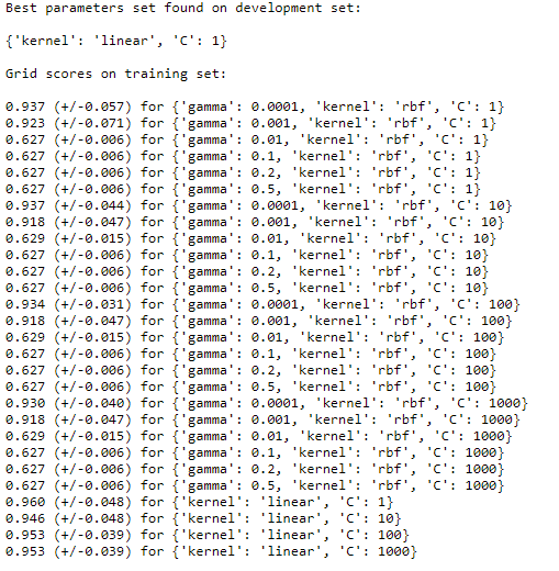
With the help of this, we can see and find out which combination of parameters is giving us the better result.

Here, the best combination turns out to be a linear kernel with a C value of 1.