
Thou, nature, art my goddess; to thy laws my services are bound. …
CARL F. GAUSS
We shall now pick up the threads of the development of differential geometry, particularly the theory of surfaces as founded by Euler and extended by Monge. The next great step in this subject was made by Gauss.
Gauss had devoted an immense amount of work to geodesy and map-making starting in 1816. His participation in actual physical surveys, on which he published many papers, stimulated his interest in differential geometry and led to his definitive 1827 paper “Disquisitiones Generales circa Superficies Curvas” (General Investigations of Curved Surfaces).1 However, beyond contributing this definitive treatment of the differential geometry of surfaces lying in three-dimensional space Gauss advanced the totally new concept that a surface is a space in itself. It was this concept that Riemann generalized, thereby opening up new vistas in non-Euclidean geometry.
Euler had already introduced the idea (Chap. 23, sec. 7) that the coordinates (x, y, z) of any point on a surface can be represented in terms of two parameters u and v; that is, the equations of a surface are given by
Gauss’s point of departure was to use this parametric representation for the systematic study of surfaces. From these parametric equations we have

wherein a = xu, a′ = xv, and so forth. For convenience Gauss introduces the determinants
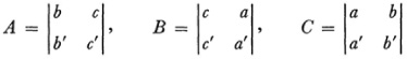
and the quantity
which he supposes is not identically 0.
The fundamental quantity on any surface is the element of arc length which in (x, y, z) coordinates is

Gauss now uses the equations (2) to write (3) as

where

The angle between two curves on a surface is another fundamental quantity. A curve on the surface is determined by a relation between u and v, for then x, y, and z become functions of one parameter, u or v, and the equations (1) become the parametric representation of a curve. One says in the language of differentials that at a point (u, v) a curve or the direction of a curve emanating from the point is given by the ratio du: dv. If then we have two curves or two directions emanating from (u, v), one given by du′: dv′ and the other by du′: dv′, and if θ is the angle between these directions, Gauss shows that

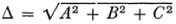
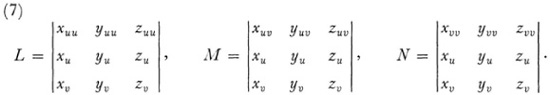
Gauss undertakes next to study the curvature of a surface. His definition of curvature is a generalization to surfaces of the indicatrix used for space curves by Euler and used for surfaces by Olinde Rodrigues.2 At each point (x, y, z) on a surface there is a normal with a direction attached. Gauss considers a unit sphere and chooses a radius having the direction of the directed normal on the surface. The choice of radius determines a point (X, Y, Z) on the sphere. If we next consider on the surface any small region surrounding (x, y, z) then there is a corresponding region on the sphere surrounding (X, Y, Z). The curvature of the surface at (x, y, z) is defined as the limit of the ratio of the area of the region on the sphere to the area of the corresponding region on the surface as the two areas shrink to their respective points. Gauss evaluates this ratio by noting first that the tangent plane at (X, Y, Z) on the sphere is parallel to the one at (x, y, z) on the surface. Hence the ratio of the two areas is the ratio of their projections on the respective tangent planes. To find this latter ratio Gauss performs an amazing number of differentiations and obtains a result which is still basic, namely, that the (total) curvature K of the surface is
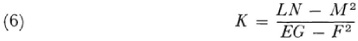
wherein
Then Gauss shows that his K is the product of the two principal curvatures at (x, y, z), which had been introduced by Euler. The notion of mean curvature, the average of the two principal curvatures, was introduced by Sophie Germain in 1831.3
Now Gauss makes an extremely important observation. When the surface is given by the parametric equations (1), the properties of the surface seem to depend on the functions x, y, z. By fixing u, say u = 3, and letting v vary, one obtains a curve on the surface. For the various possible fixed values of u one obtains a family of curves. Likewise by fixing v one obtains a family of curves. These two families are the parametric curves on the surface so that each point is given by a pair of numbers (c, d), say, where u = c and v = d are the parametric curves which pass through the point. These coordinates do not necessarily denote distances any more than latitude and longitude do. Let us think of a surface on which the parametric curves have been determined in some way. Then, Gauss affirms, the geometrical properties of the surface are determined solely by the E, F, and G in the expression (4) for ds2. These functions of u and v are all that matter.
It is certainly the case, as is evident from (4) and (5), that distances and angles on the surface arc determined by the E, F, and G. But Gauss’s fundamental expression for curvature, (6) above, depends upon the additional quantities L, M, and N. Gauss now proves that

wherein  and is equal to Gauss’s Δ defined above. Equation (8), called the Gauss characteristic equation, shows that the curvature K and, in particular in view of (6), the quantity LN – M2 depend only upon E, F, and G. Since E, F, and G are functions only of the parametric coordinates on the surface, the curvature too is a function only of the parameters and does not depend at all on whether or how the surface lies in three-space.
Gauss had made the observation that the properties of a surface depend only on E, F, and G. However, many properties other than curvature involve the quantities L, M, and N and not in the combination LN – M2 which appears in equation (6). The analytical substantiation of Gauss’s point was made by Gaspare Mainardi (1800-79),4 and independently by Delfino Codazzi (1824-75),5 both of whom gave two additional relations in the form of differential equations which together with Gauss’s characteristic equation, K having the value in (6), determine L, M, and N in terms of E, F, and G.
Then Ossian Bonnet (1819-92) proved in 1867 6 the theorem that when six functions satisfy the Gauss characteristic equation and the two Mainardi-Codazzi equations, they determine a surface uniquely except as to position and orientation in space. Specifically, if E, F, and G and L, M, and N are given as functions of u and v which satisfy the Gauss characteristic equation and the Mainardi-Codazzi equations and if EG – F2 ≠ 0, then there exists a surface given by three functions x, y, and z as functions of u and v which has the first fundamental form
E du2 + 2F du dv + G dv2,
and L, M, and N are related to E, F, and G through (7). This surface is uniquely determined except for position in space. (For real surfaces with real coordinates (u, v) we must have EG – F2 > 0, E > 0, and G ≥ 0). Bonnet’s theorem is the analogue of the corresponding theorem on curves (Chap. 23, sec. 6).
The fact that the properties of a surface depend only on the E, F, and G has many implications some of which were drawn by Gauss in his 1827 paper. For example, if a surface is bent without stretching or contracting, the coordinate lines u = const, and v = const, will remain the same and so ds will remain the same. Hence all properties of the surface, the curvature in particular, will remain the same. Moreover, if two surfaces can be put into one-to-one correspondence with each other, that is, if u′ = ø(u, v), v′ = ψ(u, v), where u′ and v′ are the coordinates of points on the second surface, and if the element of distance at corresponding points is the same on the two surfaces, that is, if
E du2 + 2F du dv + G dv2 = E′ du′2 + 2F′ du′ dv′ + G′ dv′2
wherein E, F, and G are functions of u and v and E′, F′, G′ are functions of u′ and v′, then the two surfaces, which are said to be isometric, must have the same geometry. In particular, as Gauss pointed out, they must have the same total curvature at corresponding points. This result Gauss called a “theorema egregium,” a most excellent theorem.
As a corollary, it follows that to move a part of a surface over to another part (which means preserving distance) a necessary condition is that the surface have constant curvature. Thus, a part of a sphere can be moved without distortion to another but this cannot be done on an ellipsoid. (However, bending can take place in fitting a surface or part of a surface onto another under an isometric mapping.) Though the curvatures at corresponding points are equal, if two surfaces do not have constant curvature they need not necessarily be isometrically related. In 18397 Ferdinand Minding (1806-85) proved that if two surfaces do have constant and equal curvature then one can be mapped isometrically onto the other.
Another topic of great importance that Gauss took up in his 1827 paper is that of finding geodesies on surfaces. (The term geodesic was introduced in 1850 by Liouville and was taken from geodesy.) This problem calls for the calculus of variations which Gauss uses. He approaches this subject by working with the x, y, z representation and proves a theorem stated by John Bernoulli that the principal normal of a geodesic curve is normal to the surface. (Thus the principal normal at a point of a latitude circle on a sphere lies in the plane of the circle and is not normal to the sphere whereas the principal normal at a point on a longitude circle is normal to the sphere.) Any relation between u and v determines a curve on the surface and the relation which gives a geodesic is determined by a differential equation. This equation, which Gauss merely says is a second order equation in u and v but does not give explicitly, can be written in many forms. One is

where n, m, μ, v, l, and λ are functions of E, F, and G.
One must be careful about assuming the existence of a unique geodesic between two points on a surface. Two nearby points on a sphere have a unique geodesic joining them, but two diametrically opposite points are joined by an infinity of geodesies. Similarly, two points on the same generator of a circular cylinder are connected by a geodesic along the generator but also by an infinite number of geodesic helices. If there is but one geodesic arc between two points in a region, that arc gives the shortest path between them in that region. The problem of actually determining the geodesies on particular surfaces was taken up by many men.
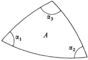
In the 1827 article Gauss proved a famous theorem on curvature for a triangle formed by geodesies (Fig. 37.1). Let K be the variable curvature of a surface. ∫∫A K dA is then the integral of this curvature over the area A. Gauss’s theorem applied to the triangle states that
that is, the integral of the curvature over a geodesic triangle is equal to the excess of the sum of the angles over 180° or, where the angle sum is less than π, to the defect from 180°. This theorem, Gauss says, ought to be counted as a most elegant theorem. The result generalizes the theorem of Lambert (Chap. 36, sec. 4), which states that the area of a spherical triangle equals the product of its spherical excess and the square of the radius, for in a spherical triangle K is constant and equals I/R2.
One more important piece of work in Gauss’s differential geometry must be noted. Lagrange (Chap. 23, sec. 8) had treated the conformai mapping of a surface of revolution into the plane. In 1822 Gauss won a prize offered by the Danish Royal Society of Sciences for a paper on the problem of finding the analytic condition for transforming any surface conformally onto any other surface.8 His condition, which holds in the neighborhood of corresponding points on the two surfaces, amounts to the fact that a function P + iQ, which we shall not specify further, of the parameters T and U by means of which one surface is represented is a function f of p + iq which is the corresponding function of the parameters t and u by which the other surface is represented and P – iQ is f′(p – iq), where f′ is f or obtained from f by replacing i by – i. The function f depends on the correspondence between the two surfaces, the correspondence being specified by T = T(i, u) and U(t, u). Gauss did not answer the question of whether and in what way a finite portion of the surface can be mapped conformally onto the other surface. This problem was taken up by Riemann in his work on complex functions (Chap. 27, sec. 10).
Gauss’s work in differential geometry is a landmark in itself. But its implications were far deeper than he himself appreciated. Until this work, surfaces had been studied as figures in three-dimensional Euclidean space. But Gauss showed that the geometry of a surface could be studied by concentrating on the surface itself. If one introduces the u and v coordinates which come from the parametric representation
x = x(u, v), y = y (u, v), z = z(u, v)
of the surface in three-dimensional space and uses the E, F, and G determined thereby then one obtains the Euclidean properties ofthat surface. However, given these u and v coordinates on the surface and the expression for ds2 in terms of E, F, and G as functions of u and v, all the properties of the surface follow from this expression. This suggests two vital thoughts. The first is that the surface can be considered as a space in itself because all its properties are determined by the ds2. One can forget about the fact that the surface lies in a three-dimensional space. What kind of geometry does the surface possess if it is regarded as a space in itself? If one takes the “straight lines” on that surface to be the geodesies, then the geometry is non-Euclidean.
Thus if the surface of the sphere is studied as a space in itself, it has its own geometry and even if the familiar latitude and longitude are used as the coordinates of points, the geometry of that surface is not Euclidean because the “straight lines” or geodesies are arcs of the great circles on the surface. However, the geometry of the spherical surface is Euclidean if it is regarded as a surface in three-dimensional space. The shortest distance between two points on the surface is then the line segment of three-dimensional Euclidean geometry (though it does not lie on the surface). What Gauss’s work implied is that there are non-Euclidean geometries at least on surfaces regarded as spaces in themselves. Whether Gauss saw this non-Euclidean interpretation of his geometry of surfaces is not clear.
One can go further. One might think that the proper E, F, and G for a surface is determined by the parametric equations (1). But one could start with the surface, introduce the two families of parametric curves and then pick functions E, F, and G of u and v almost arbitrarily. Then the surface has a geometry determined by these E, F, and G. This geometry is intrinsic to the surface and has no connection with the surrounding space.8a Consequently the same surface can have different geometries depending on the choice of the functions E, F, and G.
The implications are deeper. If one can pick different sets of E, F, and G and thereby determine different geometries on the same surface, why can’t one pick different distance functions in our ordinary three-dimensional space? The common distance function in rectangular coordinates is, of course, ds2 = dx2 + dy2 + dz2 and this is obligatory if one starts with Euclidean geometry because it is just the analytic statement of the Pythagorean theorem. However, given the same rectangular Cartesian coordinates for the points of space, one might pick a different expression for ds2 and obtain a quite different geometry for that space, a non-Euclidean geometry. This extension to any space of the ideas Gauss first obtained by studying surfaces was taken up and developed by Riemann.
The doubts about what we may believe about the geometry of physical space, raised by the work of Gauss, Lobatchevsky, and Bolyai, stimulated one of the major creations of the nineteenth century, Riemannian geometry. The creator was Georg Bernhard Riemann, the deepest philosopher of geometry. Though the details of Lobatchevsky’s and Bolyai’s work were unknown to Riemann, they were known to Gauss, and Riemann certainly knew Gauss’s doubts as to the truth and necessary applicability of Euclidean geometry. Thus in the field of geometry Riemann followed Gauss whereas in function theory he followed Cauchy and Abel. His investigation of geometry was influenced also by the teachings of the psychologist Johann Friedrich Herbart (1776-1841).
Gauss assigned to Riemann the subject of the foundations of geometry as the one on which he should deliver his qualifying lecture, the Habilitat-ionsvortrag, for the title of Privatdozent. The lecture was delivered in 1854 to the faculty at Göttingen with Gauss present, and was published in 1868 under the title “Über die Hypothesen, welche der Geometrie zu Grunde liegen” (On the Hypotheses Which Lie at the Foundation of Geometry).9
In a paper on the conduction of heat, which Riemann wrote in 1861 to compete for a prize offered by the Paris Academy of Sciences and which is often referred to as his Pariserarbeit, Riemann found the need to consider further his ideas on geometry and here he gave some technical elaborations of his 1854 paper. This 1861 paper, which did not win the prize, was published posthumously in 1876 in his Collected Works.10 In the second edition of the Werke Heinrich Weber in a note explains Riemann’s highly compressed material.
The geometry of space offered by Riemann was not just an extension of Gauss’s differential geometry. It reconsidered the whole approach to the study of space. Riemann took up the question of just what we may be certain of about physical space. What conditions or facts are presupposed in the very experience of space before we determine by experience the particular axioms that hold in physical space? One of Riemann’s objectives was to show that Euclid’s particular axioms were empirical rather than, as had been believed, self-evident truths. He adopted the analytical approach because in geometrical proofs we may be misled by our perceptions to assume facts not explicitly recognized. Thus Riemann’s idea was that by relying upon analysis we might start with what is surely a priori about space and deduce the necessary consequences. Any other properties of space would then be known to be empirical. Gauss had concerned himself with this very same problem but of this investigation only the essay on curved surfaces was published. Riemann’s search for what is a priori led him to study the local behavior of space or, in other words, the differential geometric approach as opposed to the consideration of space as a whole as one finds it in Euclid or in the non-Euclidean geometry of Gauss, Bolyai, and Lobatchevsky. Before examining the details we should be forewarned that Riemann’s ideas as expressed in the lecture and in the manuscript of 1854 are vague. One reason is that Riemann adapted it to his audience, the entire faculty at Göttingen. Part of the vagueness stems from the philosophical considerations with which Riemann began his paper.
Guided to a large extent by Gauss’s intrinsic geometry of surfaces in Euclidean space, Riemann developed an intrinsic geometry for any space. He preferred to treat n-dimensional geometry even though the three-dimensional case was clearly the important one and he speaks of n-dimensional space as a manifold. A point in a manifold of n-dimensions is represented by assigning special values to n variable parameters, x1, x2, …, xn, and the aggregate of all such possible points constitutes the n-dimensional manifold itself, just as the aggregate of the points on a surface constitutes the surface itself. The n variable parameters are called coordinates of the manifold. When the xi’s vary continuously, the points range over the manifold.
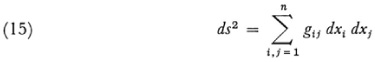
Because Riemann believed that we know space only locally he started by defining the distance between two generic points whose corresponding coordinates differ only by infinitesimal amounts. He assumes that the square of this distance is
wherein the gij are functions of the coordinates x1 x2, …, xn, gij = gji and the right side of (10) is always positive for all possible values of the dxi. This expression for ds2 is a generalization of the Euclidean distance formula
He mentions the possibility of assuming for ds the fourth root of a homogeneous function of the fourth degree in the differentials dx1 dx2, …, dxn but did not pursue this possibility. By allowing the gij to be functions of the coordinates Riemann provided for the possibility that the nature of the space may vary from point to point.
Though Riemann in his paper of 1854 did not set forth explicitly the following definitions he undoubtedly had them in mind because they parallel what Gauss did for surfaces. A curve on a Riemannian manifold is given by the set of n functions

Then the length of a curve between t = α and t = β is defined by
The shortest curve between two given points, t = α and t = β, the geodesic, is then determinable by the method of the calculus of variations. In the notation of that subject it is the curve for which  . One must then determine the particular functions of the form (11) which furnish this shortest path between the two points. In terms of the parameter arc length s, the equations of the geodesies prove to be
This is a system of n second order ordinary differential equations.11
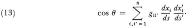
The angle θ between two curves meeting at a point (x1, x2, …, xn) one curve determined by the directions dxi/ds, i = 1, 2, …, n, and the other by , where the primes indicate values belonging to the second direction, is defined by the formula
By following the procedures which Gauss used for surfaces, a metrical n-dimensional geometry can be developed with the above definitions as a basis. All the metrical properties are determined by the coefficients gij in the expression for ds2.
The second major concept in Riemann’s 1854 paper is the notion of curvature of a manifold. Through it Riemann sought to characterize Euclidean space and more generally spaces on which figures may be moved about without change in shape or magnitude. Riemann’s notion of curvature for any n-dimensional manifold is a generalization of Gauss’s notion of total curvature for surfaces. Like Gauss’s notion, the curvature of the manifold is defined in terms of quantities determinable on the manifold itself and there is no need to think of the manifold as lying in some higher-dimensional manifold.
Given a point P in the n-dimensional manifold, Riemann considers a two-dimensional manifold at the point and in the n-dimensional manifold. Such a two-dimensional manifold is formed by a singly infinite set of geodesies through the point and tangent to a plane section of the manifold through the point P. Now a geodesic can be described by the point P and a direction at that point. Let  be the direction of one geodesic and
  be the direction of another. Then the ith direction of any one of the singly infinite set of geodesies at P is given by
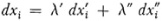
(subject to the condition λ′2 + λ″2 + 2λ′″ cos θ = 1 which arises from the condition 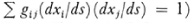 . This set of geodesies forms a two-dimensional manifold which has a Gaussian curvature. Because there is an infinity of such two-dimensional manifolds through P we obtain an infinite number of curvatures at that point in the n-dimcnsional manifold. But from n(n — l)/2 of these measures of curvature, the rest can be deduced. An explicit expression for the measure of curvature can now be derived. This was done by Riemann in his 1861 paper and will be given below. For a manifold which is a surface, Riemann’s curvature is exactly Gauss’s total curvature. Strictly speaking, Riemann’s curvature, like Gauss’s, is a property of the metric imposed on the manifold rather than of the manifold itself.
After Riemann had completed his general investigation of n-dimensional geometry and showed how curvature is introduced, he considered more restricted manifolds on which finite spatial forms must be capable of movement without change of size or shape and must be capable of rotation in any direction. This led him to spaces of constant curvature.
When all the measures of curvature at a point are the same and equal to all the measures at any other point, we get what Riemann calls a manifold of constant curvature. On such a manifold it is possible to treat congruent figures. In the 1854 paper Riemann gave the following results but no details: If α be the measure of curvature the formula for the infinitesimal element of distance on a manifold of constant curvature becomes (in a suitable coordinate system)
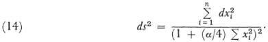
Riemann thought that the curvature α must be positive or zero, so that when α > 0 we get a spherical space and when α = 0 we get a Euclidean space and conversely. He also believed that if a space is infinitely extended the curvature must be zero. He did, however, suggest that there might be a real surface of constant negative curvature.12
To elaborate on Riemann, for α = a2 > 0 and n = 3 we get a three-dimensional spherical geometry though we cannot visualize it. The space is finite in extent but boundless. All geodesies in it are of constant length, namely, 2π/a, and return upon themselves. The volume of the space is 2π2/a3. For a2 > 0 and n = 2 we get the space of the ordinary spherical surface. The geodesies are of course the great circles and are finite. Moreover, any two intersect in two points. Actually it is not clear whether Riemann regarded the geodesies of a surface of constant positive curvature as cutting in one or two points. He probably intended the latter. Felix Klein pointed out later (see the next chapter) that there were two distinct geometries involved.
Riemann also points out a distinction, of which more was made later, between boundlessness [as is the case for the surface of a sphere] and infiniteness of space. Unboundedness, he says, has a greater empirical credibility than any other empirically derived fact such as infinite extent.
Toward the end of his paper Riemann notes that since physical space is a special kind of manifold the geometry ofthat space cannot be derived only from general notions about manifolds. The properties that distinguish physical space from other triply extended manifolds arc to be obtained only from experience. He adds, “It remains to resolve the question of knowing in what measure and up to what point these hypotheses about manifolds are confirmed by experience.” In particular the axioms of Euclidean geometry may be only approximately true of physical space. Like Lobatchevsky, Riemann believed that astronomy will decide which geometry fits space. He ends his paper with the prophetic remark: “Either therefore the reality which underlies space must form a discrete manifold or we must seek the ground of its metric relations outside it, in the binding forces which act on it… . This leads us into the domain of another science, that of physics, into which the object of our work does not allow us to go today.”
This point was developed by William Kingdon Clifford.13
I hold in fact: (1) That small portions of space arc of a nature analogous to little hills on a surface which is on the average flat. (2) That this property of being curved or distorted is continually passed on from one portion of space to another after the manner of a wave. (3) That this variation of the curvature of space is really what happens in that phenomenon which we call the motion of matter whether ponderable or ethereal. (4) That in this physical world nothing else takes place but this variation, subject, possibly, to the law of continuity.
The ordinary laws of Euclidean geometry are not valid for a space whose curvature changes not only from place to place but because of the motion of matter, from time to time. He added that a more exact investigation of physical laws would not be able to ignore these “hills” in space. Thus Riemann and Clifford, unlike most other geometers, felt the need to associate matter with space in order to determine what is true of physical space. This line of thought leads, of course, to the theory of relativity.
In his Pariserarbeit (1861) Riemann returned to the question of when a given Riemannian space whose metric is
might be a space of constant curvature or even a Euclidean space. However, he formulated the more general question of when a metric such as (15) can be transformed by the equations

into a given metric
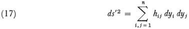
with the understanding of course that ds would equal ds′ so that the geometries of the two spaces would be the same except for the choice of coordinates. The transformation (16) is not always possible because, as Riemann points out, there are n(n + 1)/2 independent functions in (15), whereas the transformation introduces only n functions which might be used to convert the gij into the hij.
To treat the general question Riemann introduced special quantities pijk which we shall replace by the more familiar Christoffel symbols with the understanding that

The Christoffel symbols, denoted in various ways, are

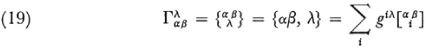
where giλ is the cofactor divided by g of giλ in the determinant of g. Riemann also introduced what is now known as the Riemann four index symbol

Then Riemann shows that a necessary condition that ds2 be transformable to ds′2 is
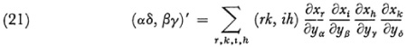
where the left-hand symbol refers to quantities formed for the ds′ metric and (21) holds for all values of α, β, γ, δ, each of which ranges from 1 to n.
And now Riemann turns to the specific question of when a given ds2 can be transformed to one with constant coefficients. He first derives an explicit expression for the curvature of a manifold. The general definition already given in the 1854 paper makes use of the geodesic lines issuing from a point O of the space. Let d and δ determine two vectors or directions of geodesies emanating from O. (Each direction is specified by the components of the tangent to the geodesic.) Then consider the pencil of geodesic vectors emanating from O and given by κd + λδ where κ and λ are parameters. If one thinks of d and δ as operating on the xi = fi(t) which describe any one curve, then there is a meaning for the second differential (κd + λδ)2 = κ2d2 + 2κλdδ + λ2δ2. Riemann then forms

Here one understands that the d and δ operate formally on the expressions following them (and d and δ commute) so that

and δgij = Σr(∂gij/∂xi) If one calculates Ω one finds that all terms involving third differentials of a function vanish. Only terms involving δxi, dxi, δ2xi, δdxi, and d2xi remain. By calculating these terms and by using the notation
Pik = dxi δxκ – dxκ δxi
Riemann obtains
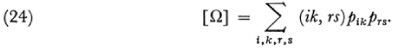
Now let

Then the curvature K of a Riemannian manifold is
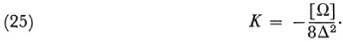
The overall conclusion is that the necessary and sufficient condition that a given ds2 can be brought to the form (for n = 3)

where the ci’s are constants, is that all the symbols (αβ, γδ) be zero. In case the ci’s are all positive the ds′ can be reduced to  , that is, the space is Euclidean. As we can see from the value of [Ω], when K is zero, the space is essentially Euclidean.
It is worth noting that Riemann’s curvature for an n-dimensional manifold reduces to Gauss’s total curvature of a surface. In fact when

of the 16 symbols (αβ, γδ), 12 are zero and for the remaining four we have (12, 12) = –(12, 21) = –(21, 12) = (21, 21). Then Riemann’s K reduces to
By using (20) this expression can be shown to be equal to Gauss’s expression for the total curvature of a surface.
When Riemann’s essay of 1854 was published in 1868, two years after his death, it created intense interest, and many mathematicians hastened to fill in the ideas he sketched and to extend them. The immediate successors of Riemann were Beltrami, Christoffel, and Lipschitz.
Eugenio Beltrami (1835-1900), professor of mathematics at Bologna and other Italian universities, who knew Riemann’s 1854 paper but apparently did not know his 1861 paper, took up the matter of proving that the general expression for ds2 reduces to the form (14) given by Riemann for a space of constant curvature.14 Beyond this result and proving a few other assertions by Riemann, Beltrami took up the subject of differential invariants, which we shall consider in the next section.
Elwin Bruno Christoffel (1829-1900), who was a professor of mathematics at Zurich and later at Strasbourg, advanced the ideas in both of Riemann’s papers. In two key papers15 Christoffel’s major concern was to reconsider and amplify the theme already treated somewhat sketchily by Riemann in his 1861 paper, namely, when one form
can be transformed into another
Christoffel sought necessary and sufficient conditions. It was in this paper, incidentally, that he introduced the Christoffel symbols.
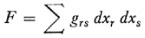
Let us consider first the two-dimensional case where
F = a dx2 + 2b dx dy + c dy2
and
F′ = A dX2 + 2B dX dY + C dY2
and suppose that x and y may be expressed as functions of X and Y so that F becomes F′ under the transformation. Of course dx = (∂x/∂X) dX + (∂x/∂Y) dY. Now when x, y, dx, and dy are replaced in F by their values in X and Y and when one equates coefficients in this new form of F with those of F′ one obtains
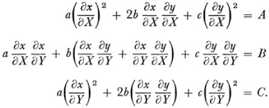
These are three differential equations for x and y as functions of X and Y. If they can be solved then we know how to transform from F to F′. However, there are only two functions involved. There must then be some relations between a, b, and c on the one hand and A, B, and C on the other. By differentiating the three equations above and further algebraic steps the relation proves to be K = K′.
For the n-variable case, Christoffel uses the same technique. He starts with
and
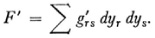
The transformation is
xi = xi(y1, y2, …, yn), i = 1, 2, …, n.
He lets g = |grs|. Then if Δrs is the cofactor of grs in the determinant let gpq = Δpq/g. He, like Riemann, introduces independently the four index symbol (without the comma)

He then deduces n(n + l)/2 partial differential equations for the xi as functions of the yi. A typical one is
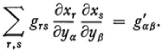
These equations are the necessary and sufficient conditions that a transformation exist for which F = F′.
Partly to treat the integrability of this set of equations and partly because Christoffel wishes to consider forms of degree higher than two in the dxi he performs a number of differentiations and algebraic steps which show that
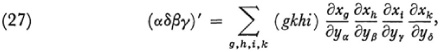
where α, β, γ, and δ take all values from 1 to n. There are n2(n2 – 1)/12 equations of this form. These equations are the necessary and sufficient conditions for the equivalence of two differential forms of fourth order. Indeed let d(1)x, d(2)x, d(3)x, d(4)x, be four sets of differentials of x and likewise for the y′s. Then if we have the quadrilinear form
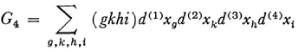
the relations (27) are necessary and sufficient that  , where
  is the analogue of G4 in the y variables.
This theory can be generalized to μ-ply differential forms. In fact Christoffel introduces
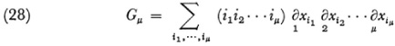
where the term in parentheses is defined in terms of the grs much as the four index symbol is and the symbol ∂ is used to distinguish the differentials of the set of xi from the set obtained by applying ∂. He then shows that
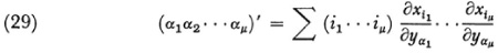
and obtains necessary and sufficient conditions that Gμ be transformable into  .
.
He gives next a general procedure whereby from a μ-ply form Gμ a (μ + l)-ply form Gμ + 1 can be derived. The key step is to introduce
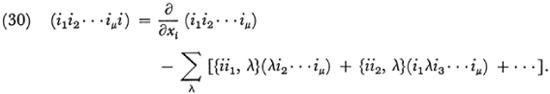
These (μ + 1)-index symbols are the coefficients of the Gμ + 1 form. The procedure Christoffel uses here is what Ricci and Levi-Civita later called covariant differentiation (Chap. 48).
Whereas Christoffel wrote only one key paper on Riemannian geometry, Rudolph Lipschitz, professor of mathematics at Bonn University, wrote a great number appearing in the Journal für Mathematik from 1869 on. Though there are some generalizations of the work of Beltrami and Christoffel, the essential subject matter and results are the same as those of the latter two men. He did produce some new results on subspaces of Riemannian and Euclidean n-dimensional spaces.
The ideas projected by Riemann and developed by his three immediate successors suggested hosts of new problems in both Euclidean and Riemannian differential geometry. In particular the results already obtained in the Euclidean case for three dimensions were generalized to curves, surfaces, and higher-dimensional forms in n dimensions. Of many results we shall cite just one.
In 1886 Friedrich Schur (1856-1932) proved the theorem named after him.16 In accordance with Riemann’s approach to the notion of curvature, Schur speaks of the curvature of an orientation of space. Such an orientation is determined by a pencil of geodesies μα + λβ where α and β are the directions of two geodesies issuing from a point. This pencil forms a surface and has a Gauss curvature which Schur calls the Riemannian curvature of that orientation. His theorem then states that if at each point the Riemannian curvature of a space is independent of the orientation then the Riemannian curvature is constant throughout the space. The manifold is then a space of constant curvature.
It was clear from the study of the question of when a given expression for ds2 can be transformed by a transformation of the form

to another such expression with preservation of the value of ds2 that different coordinate representations can be obtained for the very same manifold. However, the geometrical properties of the manifold must be independent of the particular coordinate system used to represent and study it. Analytically these geometrical properties would be represented by invariants, that is, expressions which retain their form under the change of coordinates and which will consequently have the same value at a given point. The invariants of interest in Riemannian geometry involve not only the fundamental quadratic form, which contains the differentials dxi and dxj, but may also contain derivatives of the coefficients and of other functions. They are therefore called differential invariants.
To use the two-dimensional case as an example, if

is the element of distance for a surface then the Gaussian curvature K is given by formula (8) above. If now the coordinates are changed to

then there is the theorem that if E du2 + 2F du dv + G dv2 transforms into E′ du′2 + 2F′ du′ dv′ + G′ dv′2 then K = K′, where K′ is the same expression as in (8) but in the accented variables. Hence the Gaussian curvature of a surface is a scalar invariant. The invariant K is said to be an invariant attached to the form (32) and involves only E, F, and G and their derivatives.
The study of differential invariants was actually initiated in a more limited context by Lamé. He was interested in invariants under transformations from one orthogonal curvilinear coordinate system in three dimensions to another. For rectangular Cartesian coordinates he showed17 that
are differential invariants (he called them differential parameters). Thus if ø is transformed into ø′(x′, y′, z′) under an orthogonal transformation (rotation of axes) then
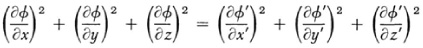
at the same point whose coordinates are (x, y, z) in the original system and (x′, y′, z′) in the new coordinate system. The analogous equation holds for  .
.
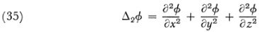
For orthogonal curvilinear coordinates in Euclidean space where ds2 has the form

Lamé showed (Leçons sur les coordonnées curvilignes, 1859, cf. above Chapter 28, sec. 5) that the divergence of the gradient of ø, which in rectangular coordinates is given by above, has the invariant form
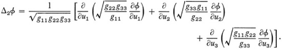
Incidentally in this same work Lamé gave conditions on when the ds2 given by (36) determines a curvilinear coordinate system in Euclidean space and, if it does, how to change to rectangular coordinates.
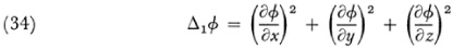
The investigation of invariants for the theory of surfaces was first made by Beltrami.18 He gave the two differential invariants
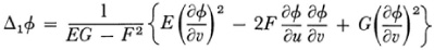
and

These have geometrical meaning. For example in the case of Δ1ø, if Δ1ø = 1, the curves ø(u, v) = const, are the orthogonal trajectories of a family of geodesies on the surface.
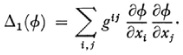
The search for differential invariants was carried over to quadratic differential forms in n variables. The reason again was that these invariants are independent of particular choices of coordinates; they represent intrinsic properties of the manifold itself. Thus the Riemann curvature is a scalar invariant.
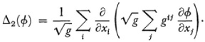
Beltrami, using a method given by Jacobi,19 succeeded in carrying over to n-dimensional Riemannian spaces the Lamé invariants.20 Let g as usual be the determinant of the gij and let gij be the cofactor divided by g of gij in g. Then Beltrami showed that Lamé’s first invariant becomes
This is the general form for the square of the gradient of ø. For the second of Lamé’s invariants Beltrami obtained
He also introduced the mixed differential invariant
This is the general form of the scalar product of the gradients of ø and ψ.
Of course the form ds2 is itself an invariant under a change of coordinates. From this, as we found in the previous section, Christoffel derived higher order differential forms, his G4 and Gu, which are also invariants. Moreover, he showed how from Gμ one can derive Gμ + 1 which is also an invariant. The construction of such invariants was also pursued by Lipschitz. The number and variety are extensive. As we shall see this theory of differential invariants was the inspiration for tensor analysis.
Beltrami, Eugenio: Opere matematiche, 4 vols., Ulrico Hoepli, 1902-20.
Clifford, William K.: Mathematical Papers, Macmillan, 1882; Chelsea (reprint), 1968.
Coolidge, Julian L.: A History of Geometrical Methods, Dover (reprint), 1963, pp. 355-87.
Enzyklopädie der Mathematischen Wissenschaften, III, Teil 3, various articles, B. G. Teubner, 1902-7.
Gauss, Carl F.: Werke, 4, 192-216, 217-58, Königliche Gesellschaft der Wissenschaften zu Göttingen, 1880. A translation, “General Investigations of Curved Surfaces,” has been reprinted by Raven Press, 1965.
Helmholtz, Hermann von: “Über die tatsächlichen Grundlagen der Geometrie,” Wissenschaftliche Abhandlungen, 2, 610-17.
——: “Über die Tatsachen, die der Geometrie zum Grunde liegen,” Nachrichten König. Ges. der Wiss. zu Gött., 15, 1868, 193-221; Wiss. Abh., 2, 618-39.
——: “Über den Ursprung Sinn und Bedeutung der geometrischen Sätze”; English translation, “On the Origin and Significance of Geometrical Axioms,” in Helmholtz: Popular Scientific Lectures, Dover (reprint), 1962, 223-49. Also in James R. Newman: The World of Mathematics, Simon and Schuster, 1956, Vol. 1, 647-68.
Jammer, Max: Concepts of Space, Harvard University Press, 1954.
Killing, W.: Die nicht-euklidischen Raumformen in analytischer Behandlung, B. G. Teubner, 1885.
Klein, F.: Vorlesungen über die Entwicklung der Mathematik im 19. Jahrhundert, Chelsea (reprint), 1950, Vol. 1, 6-62; Vol. 2, 147-206.
Pierpont, James: “Some Modern Views of Space,” Amer. Math. Soc. Bull., 32, 1926, 225-58.
Riemann, Bernhard: Gesammelte mathematische Werke, 2nd ed., Dover (reprint), 1953, pp. 272-87 and 391-404.
Russell, Bertrand: An Essay on the Foundations of Geometry (1897), Dover (reprint), 1956.
Smith, David E.: A Source Book in Mathematics, Dover (reprint), 1959, Vol. 2, 411-25, 463-75. This contains translations of Riemann’s 1854 paper and Gauss’s 1822 paper.
Staeckel, P.: “Gauss als Geometer,” Nachrichten König. Ges. der Wiss. zu Gött., 1917, Beiheft, 25-140; also in Werke, 102.
Weatherburn, C. E.: “The Development of Multidimensional Differential Geometry,” Australian and New Zealand Ass’n for the Advancement of Science, 21, 1933, 12-28.