
But it would be a serious error to think that one can find certainty only in geometrical demonstrations or in the testimony of the senses.
A. L. CAUCHY
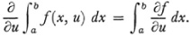
By about 1800 the mathematicians began to be concerned about the looseness in the concepts and proofs of the vast branches of analysis. The very concept of a function was not clear; the use of series without regard to convergence and divergence had produced paradoxes and disagreements; the controversy about the representations of functions by trigonometric series had introduced further confusion; and, of course, the fundamental notions of derivative and integral had never been properly defined. All these difficulties finally brought on dissatisfaction with the logical status of analysis.
Abel, in a letter of 1826 to Professor Christoffer Hansteen,1 complained about “the tremendous obscurity which one unquestionably finds in analysis. It lacks so completely all plan and system that it is peculiar that so many men could have studied it. The worst of it is, it has never been treated stringently. There are very few theorems in advanced analysis which have been demonstrated in a logically tenable manner. Everywhere one finds this miserable way of concluding from the special to the general and it is extremely peculiar that such a procedure has led to so few of the so-called paradoxes.”
Several mathematicians resolved to bring order out of chaos. The leaders of what is often called the critical movement decided to rebuild analysis solely on the basis of arithmetical concepts. The beginnings of the movement coincide with the creation of non-Euclidean geometry. An entirely different group, except for Gauss, was involved in the latter activity and it is therefore difficult to trace any direct connection between it and the decision to found analysis on arithmetic. Perhaps the decision was reached because the hope of grounding analysis on geometry, which many seventeenth-century men often asserted could be done, was blasted by the increasing complexity of the eighteenth-century developments in analysis. However, Gauss had already expressed his doubts as to the truth of Euclidean geometry as early as 1799, and in 1817 he decided that truth resided only in arithmetic. Moreover, during even the early work by Gauss and others on non-Euclidean geometry, flaws in Euclid’s development had already been noted. Hence it is very likely that both factors caused distrust of geometry and prompted the decision to found analysis on arithmetical concepts. This certainly was what the leaders of the critical movement undertook to do.
Rigorous analysis begins with the work of Bolzano, Cauchy, Abel, and Dirichlet and was furthered by Weierstrass. Cauchy and Weierstrass are best known in this connection. Cauchy’s basic works on the foundations of analysis are his Cours d’analyse algébrique,2 Résumé des leçons sur le calcul infinitésimal,3 and Leçons sur le calcul différentiel.’4 Actually Cauchy’s rigor in these works is loose by modern standards. He used phrases such as “approach indefinitely,” “as little as one wishes,” “last ratios of infinitely small increments,” and “a variable approaches its limit.” However, if one compares Lagrange’s Théorie des fonctions analytiques5 and his Leçons sur le calcul des fonctions6 and the influential book by Lacroix, Traité du calcul différentiel et du calcul intégral7 with the Cours d’analyse algébrique of Cauchy one begins to see the striking difference between the mathematics of the eighteenth century and that of the nineteenth. Lagrange, in particular, was purely formal. He operated with symbolic expressions. The underlying concepts of limit, continuity, and so on are not there.
Cauchy is very explicit in his introduction to the 1821 work that he seeks to give rigor to analysis. He points out that the free use for all functions of the properties that hold for algebraic functions, and the use of divergent series are not justified. Though Cauchy’s work was but one step in the direction of rigor, he himself believed and states in his Résumé that he had brought the ultimate in rigor into analysis. He did give the beginnings of precise proofs of theorems and properly limited assertions at least for the elementary functions. Abel in his paper of 1826 on the binomial series (sec. 5) praised this achievement of Cauchy: “The distinguished work [the Cours d’analyse] should be read by everyone who loves rigor in mathematical investigations.” Cauchy abandoned the explicit representations of Euler and the power series of Lagrange and introduced new concepts to treat functions.
The eighteenth century mathematicians had on the whole believed that a function must have the same analytic expression throughout. During the latter part of the century, largely as a consequence of the controversy over the vibrating-string problem, Euler and Lagrange allowed functions that have different expressions in different domains and used the word continuous where the same expression held and discontinuous at points where the expression changed form (though in the modern sense the entire function could be continuous). While Euler, d’Alembert, and Lagrange had to reconsider the concept of function, they did not arrive at any widely accepted definition nor did they resolve the problem of what functions could be represented by trigonometrical series. However, the gradual expansion in the variety and use of functions forced mathematicians to accept a broader concept.
Gauss in his earlier work meant by a function a closed (finite analytical) expression and when he spoke of the hypergeometric series F (α, β, γ, x) as a function of α, β, γ, and x he qualified it by the remark, “insofar as one can regard it as a function.” Lagrange had already used a broader concept in regarding power series as functions. In the second edition of his Mécanique analytique (1811-15) he used the word function for almost any kind of dependence on one or more variables. Even Lacroix in his Traité of 1797 had already introduced a broader notion. In the introduction he says, “Every quantity whose value depends on one or several others is called a function of the latter, whether one knows or one does not know by what operations it is necessary to go from the latter to the first quantity.” Lacroix gives as an example a root of an equation of the fifth degree as a function of its coefficients.
Fourier’s work opened up even more widely the question of what a function is. On the one hand, he insisted that functions need not be representable by any analytic expressions. In his The Analytical Theory of Heat8 he says, “In general the function f(x) represents a succession of values or ordinates each of which is arbitrary…. We do not suppose these ordinates to be subject to a common law; they succeed each other in any manner whatever. …” Actually he himself treated only functions with a finite number of discontinuities in any finite interval. On the other hand, to a certain extent Fourier was supporting the contention that a function must be representable by an analytic expression, though this expression was a Fourier series. In any case Fourier’s work shook the eighteenth-century belief that all functions were at worst extensions of algebraic functions. The algebraic functions and even the elementary transcendental functions were no longer the prototype of functions. Since the properties of algebraic functions could no longer be carried over to all functions, the question then arose as to what one really means by a function, by continuity, differentiability, integrability, and other properties.
In the positive reconstructions of analysis which many men undertook the real number system was taken for granted. No attempt was made to analyze this structure or to build it up logically. Apparently the mathematicians felt they were on sure ground as far as this area was concerned.
Cauchy begins his 1821 work with the definition of a variable. “One calls a quantity which one considers as having to successively assume many values different from one another a variable.” As for the concept of function, “When variable quantities are so joined between themselves that, the value of one of these being given, one may determine the values of all the others, one ordinarily conceives these diverse quantities expressed by means of the one among them, which then takes the name independent variable; and the other quantities expressed by means of the independent variable are those which one calls functions of this variable.” Cauchy is also explicit that an infinite series is one way of specifying a function. However, an analytical expression for a function is not required.
In a paper on Fourier series which we shall return to later, “Über die Darstellung ganz willkürlicher Functionen durch Sinus-und Cosinusreihen” (On the Representation of Completely Arbitrary Functions by Sine and Cosine Series),9 Dirichlet gave the definition of a (single-valued) function which is now most often employed, namely, that y is a function of A: when to each value of x in a given interval there corresponds a unique value of y. He added that it does not matter whether throughout this interval y depends upon x according to one law or more or whether the dependence of y on x can be expressed by mathematical operations. In fact in 182910 he gave the example of a function of x which has the value c for all rational values of x and the value d for all irrational values of x.
Hankel points out that the best textbooks of at least the first half of the century were at a loss as to what to do about the function concept. Some defined a function essentially in Euler’s sense; others required that y vary with x according to some law but did not explain what law meant; some used Dirichlet’s definition; and still others gave no definition. But all deduced consequences from their definitions which were not logically implied by the definitions.
The proper distinction between continuity and discontinuity gradually emerged. The careful study of the properties of functions was initiated by Bernhard Bolzano (1781-1848), a priest, philosopher, and mathematician of Bohemia. Bolzano was led to this work by trying to give a purely arithmetical proof of the fundamental theorem of algebra in place of Gauss’s first proof (1799) which used geometric ideas. Bolzano had the correct concepts for the establishment of the calculus (except for a theory of real numbers), but his work went unnoticed for half a century. He denied the existence of infinitely small numbers (infinitesimals) and infinitely large numbers, both of which had been used by the eighteenth-century writers. In a book of 1817 whose long title starts with Rein analytischer Beweis (see the bibliography) Bolzano gave the proper definition of continuity, namely, f(x) is continuous in an interval if at any x in the interval the difference f(x + ω) – f(x) can be made as small as one wishes by taking ω sufficiently small. He proves that polynomials are continuous.
Cauchy, too, tackled the notions of limit and continuity. As with Bolzano the limit concept was based on purely arithmetical considerations. In the Cours (1821) Cauchy says, “When the successive values attributed to a variable approach indefinitely a fixed value so as to end by differing from it by as little as one wishes, this last is called the limit of all the others. Thus, for example, an irrational number is the limit of diverse fractions which furnish closer and closer approximate values of it.” This example was a bit unfortunate because many took it to be a definition of irrational numbers in terms of limit whereas the limit could have no meaning if irrationals were not already present. Cauchy omitted it in his 1823 and 1829 works.
In the preface to his 1821 work Cauchy says that to speak of the continuity of functions he must make known the principal properties of infinitely small quantities. “One says [Cours, p. 5] that a variable quantity becomes infinitely small when its numerical value decreases indefinitely in such a way as to converge to the limit 0.” Such variables he calls infinitesimals. Thus Cauchy clarifies Leibniz’s notion of infinitesimal and frees it of metaphysical ties. Cauchy continues, “One says that a variable quantity becomes infinitely large when its numerical value increases indefinitely in such a manner as to converge to the limit ∞.” However, ∞ means not a fixed quantity but something indefinitely large.
Cauchy is now prepared to define continuity of a function. In the Cours (pp. 34-35) he says. “Let f(x) be a function of the variable x, and suppose that, for each value of x intermediate between two given limits [bounds], this function constantly assumes a finite and unique value. If, beginning with a value of x contained between these limits, one assigns to the variable x an infinitely small increment α, the function itself will take on as an increment the difference f(x + α) – f(x) which will depend at the same time on the new variable α and on the value of x. This granted, the function f(x) will be, between the two limits assigned to the variable x, a continuous function of the variable if, for each value of x intermediate between these two limits, the numerical value of the difference f(x + α) – f(x) decreases indefinitely with that of α. In other words, the function f(x) will remain continuous with respect to x between the given limits, if, between these limits, an infinitely small increment of the variable always produces an infinitely small increment of the function itself.
“We also say that the function f(x) is a continuous function of x in the neighborhood of a particular value assigned to the variable x, as long as it [the function] is continuous between those two limits of x, no matter how close together, which enclose the value in question.” He then says that f(x) is discontinuous at x0 if it is not continuous in every interval around x0.
In his Cours (p. 37) Cauchy asserted that if a function of several variables is continuous in each one separately it is a continuous function of all the variables. This is not correct.
Throughout the nineteenth century the notion of continuity was explored and mathematicians learned more about it, sometimes producing results that astonished them. Darboux gave an example of a function which took on all intermediate values between two given values in passing from x = a to x = b but was not continuous. Thus a basic property of continuous functions is not sufficient to insure continuity.11
Weierstrass’s work on the rigorization of analysis improved on Bolzano, Abel, and Cauchy. He, too, sought to avoid intuition and to build on arithmetical concepts. Though he did this work during the years 1841-56 when he was a high-school teacher much of it did not become known until 1859 when he began to lecture at the University of Berlin.
Weierstrass attacked the phrase “a variable approaches a limit,” which unfortunately suggests time and motion. He interprets a variable simply as a letter standing for any one of a set of values which the letter may be given. Thus motion is eliminated. A continuous variable is one such that if x0 is any value of the set of values of the variable and δ any positive number there are other values of the variable in the interval (x0 – δ, x0 + δ).
To remove the vagueness in the phrase “becomes and remains less than any given quantity,” which Bolzano and Cauchy used in their definitions of continuity and limit of a function, Weierstrass gave the now accepted definition that f(x) is continuous at x = x0 if given any positive number ε, there exists a δ such that for all x in the interval |x – x0| < δ, |f(x) – f(x0)| < ε. A function f(x) has a limit L at x = x0 if the same statement holds but with L replacing f(x0). A function f(x) is continuous in an interval of x values if it is continuous at each x in the interval.
During the years in which the notion of continuity itself was being refined, the efforts to establish analysis rigorously called for the proof of many theorems about continuous functions which had been accepted intuitively. Bolzano in his 1817 publication sought to prove that if f(x) is negative for x = a and positive for x = b, then f(x) has a zero between a and b. He considered the sequence of functions (for fixed x)
and introduced the theorem that if for n large enough we can make the difference Fn+r – Fn less than any given quantity, no matter how large r is, then there exists a fixed magnitude X such that the sequence comes closer and closer to X, and indeed as close as one wishes. His determination of the quantity X was somewhat obscure because he did not have a clear theory of the real number system and of irrational numbers in particular on which to build. However, he had the idea of what we now call the Cauchy condition for the convergence of a sequence (see below).
In the course of the proof Bolzano established the existence of a least upper bound for a bounded set of real numbers. His precise statement is: If a property M does not apply to all values of a variable quantity x, but to all those that are smaller than a certain u, there is always a quantity U which is the largest of those of which it can be asserted that all smaller x possess the property M. The essence of Bolzano’s proof of this lemma was to divide the bounded interval into two parts and select a particular part containing an infinite number of members of the set. He then repeats the process until he closes down on the number which is the least upper bound of the given set of real numbers. This method was used by Weierstrass in the 1860s, with due credit to Bolzano, to prove what is now called the Weierstrass-Bolzano theorem. It establishes for any bounded infinite set of points the existence of a point such that in every neighborhood of it there are points of the set.
Cauchy had used without proof (in one of his proofs of the existence of roots of a polynomial) the existence of a minimum of a continuous function defined over a closed interval. Weierstrass in his Berlin lectures proved for any continuous function of one or more variables defined over a closed bounded domain the existence of a minimum value and a maximum value of the function.
In work inspired by the ideas of Georg Cantor and Weierstrass, Heine defined uniform continuity for functions of one or several variables12 and then proved13 that a function which is continuous on a closed bounded interval of the real numbers is uniformly continuous. Heine’s method introduced and used the following theorem: Let a closed interval [a, b] and a countably infinite set Δ of intervals, all in [a, b], be given such that every point x of a ≤ x ≤ b is an interior point of at least one of the intervals of Δ. (The endpoints a and b are regarded as interior points when a is the left-hand end of an interval and b the right-hand end of another interval.) Then a set consisting of a finite number of the intervals of Δ has the same property, namely, every point of the closed interval [a, b] is an interior point of at least one of this finite set of intervals (a and b can be endpoints).
Emile Borei (1871-1956), one of the leading French mathematicians of this century, recognized the importance of being able to select a finite number of covering intervals and first stated it as an independent theorem for the case when the original set of intervals Δ is countable.14 Though many German and French mathematicians refer to this theorem as Borel’s, since Heine used the property in his proof of uniform continuity the theorem is also known as the Heine-Borei theorem. The merit of the theorem, as Lebesgue pointed out, is not in the proof of it, which is not difficult, but in perceiving its importance and enunciating it as a distinct theorem. The theorem applies to closed sets in any number of dimensions and is now basic in set theory.
The extension of the Heine-Borei theorem to the case where a finite set of covering intervals can be selected from an uncountably infinite set is usually credited to Lebesgue who claimed to have known the theorem in 1898 and published it in his Leçons sur l’intégration (1904). However, it was first published by Pierre Cousin (1867-1933) in 1895.15
D’Alembert was the first to see that Newton had essentially the correct notion of the derivative. D’Alembert says explicitly in the Encyclopédie that the derivative must be based on the limit of the ratio of the differences of dependent and independent variables. This version is a reformulation of Newton’s prime and ultimate ratio. D’Alembert did not go further because his thoughts were still tied to geometric intuition. His successors of the next fifty years still failed to give a clear definition of the derivative. Even Poisson believed that there are positive numbers that are not zero, but which are smaller than any given number however small.
Bolzano was the first (1817) to define the derivative of f(x) as the quantity f′(x) which the ratio [f(x + Δx) – f(x)]/Δx approaches indefinitely closely as Δx approaches 0 through positive and negative values. Bolzano emphasized that f′(x) was not a quotient of zeros or a ratio of evanescent quantities but a number which the ratio above approached.
In his Résumé des leçons16 Cauchy defined the derivative in the same manner as Bolzano. He then unified this notion and the Leibnizian differentials by defining dx to be any finite quantity and dy to be f′(x) dx.17 In other words, one introduces two quantities dx and dy whose ratio, by definition, is f′(x). Differentials have meaning in terms of the derivative and are merely an auxiliary notion that could be dispensed with logically but are convenient as a way of thinking or writing. Cauchy also pointed out what the differential expressions used throughout the eighteenth century meant in terms of derivatives.
He then clarified the relation between Δy/Δx and f′(x) through the mean value theorem, that is, Δy = f′(x + θΔx) Δx, where 0 < θ < 1. The theorem itself was known to Lagrange (Chap. 20, sec. 7). Cauchy’s proof of the mean value theorem used the continuity of f′(x) in the interval Δx.
Though Bolzano and Cauchy had rigorized (somewhat) the notions of continuity and the derivative, Cauchy and nearly all mathematicians of his era believed and many texts “proved” for the next fifty years that a continuous function must be differentiable (except of course at isolated points such as x = 0 for y = 1/x). Bolzano did understand the distinction between continuity and differentiability. In his Funktionenlehre, which he wrote in 1834 but did not complete and publish,18 he gave an example of a continuous function which has no finite derivative at any point. Bolzano’s example, like his other works, was not noticed.19 Even if it had been published in 1834 it probably would have made no impression because the curve did not have an analytic representation, and for mathematicians of that period functions were still entities given by analytical expressions.
The example that ultimately drove home the distinction between continuity and differentiability was given by Riemann in the Habilitationsschrift, the paper of 1854 he wrote to qualify as a Privatdozent at Göttingen, “Über die Darstellbarkeit einer Function durch eine trigonometrische Reihe,” (On the Representability of a Function by a Trigonometric Series).20 (The paper on the foundations of geometry (Chap. 37, sec. 3) was given as a qualifying lecture.) Riemann defined the following function. Let (x) denote the difference between x and the nearest integer and let (x) = 0 if it is halfway between two integers. Then – 1/2 < (x) < 1/2. Now f(x) is defined as
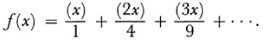
This series converges for all values of x. However, for x = p/2n where p is an integer prime to 2n, f(x) is discontinuous and has a jump whose value is π2/8n2. At all other values of x, f(x) is continuous. Moreover, f(x) is discontinuous an infinite number of times in every arbitrarily small interval. Nevertheless, f(x) is integrable (sec. 4). Moreover, F(x) = ∫ f(x) dx is continuous for all x but fails to have a derivative where f(x) is discontinuous. This pathological function did not attract much attention until it was published in 1868.
An even more striking distinction between continuity and differentiability was demonstrated by the Swiss mathematician Charles Cellérier (1818-89). In 1860 he gave an example of a function which is continuous but nowhere differentiable, namely,
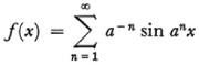
in which a is a large positive integer. This was not published, however, until 1890.21 The example that attracted the most attention is due to Weierstrass. As far back as 1861 he had affirmed in his lectures that any attempt to prove that differentiability follows from continuity must fail. He then gave the classic example of a continuous nowhere differentiable function in a lecture to the Berlin Academy on July 18, 1872.22 Weierstrass communicated his example in a letter of 1874 to Du Bois-Reymond and the example was first published by the latter.23 Weierstrass’s function is
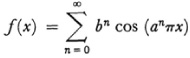
wherein a is an odd integer and b a positive constant less than I such that ab > 1 + (3π/2). The series is uniformly convergent and so defines a continuous function. The example given by Weierstrass prompted the creation of many more functions that are continuous in an interval or everywhere but fail to be differentiable either on a dense set of points or at any point.24
The historical significance of the discovery that continuity does not imply differentiability and that functions can have all sorts of abnormal behavior was great. It made mathematicians all the more fearful of trusting intuition or geometrical thinking.
Newton’s work showed how areas could be found by reversing differentiation. This is of course still the essential method. Leibniz’s idea of area and volume as a “sum” of elements such as rectangles or cylinders [the definite integral] was neglected. When the latter concept was employed at all in the eighteenth century it was loosely used.
Cauchy stressed defining the integral as the limit of a sum instead of the inverse of differentiation. There was at least one major reason for the change. Fourier, as we know, dealt with discontinuous functions, and the formula for the coefficients of a Fourier series, namely,
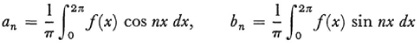
calls for the integrals of such functions. Fourier regarded the integral as a sum (the Leibnizian view) and so had no difficulty in handling even discontinuous f(x). The problem of the analytical meaning of the integral when f(x) is discontinuous had, however, to be considered.
Cauchy’s most systematic attack on the definite integral was made in his Résumé(1823) wherein he also points out that it is necessary to establish the existence of the definite integral and indirectly of the antiderivative or primitive function before one can use them. He starts with continuous functions.
For continuous f(x) he gives25 the precise definition of the integral as the limit of a sum. If the interval [x0, X] is subdivided by the x-values, x1 x2, …, xn - 1 with xn = X, then the integral is
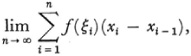
where ξi is any value of x in [xi – 1, xi]. The definition presupposes that f(x) is continuous over [x0, X] and that the length of the largest subinterval approaches zero. The definition is arithmetical. Cauchy shows the integral exists no matter how the xi and ξi are chosen. However, his proof was not rigorous because he did not have the notion of uniform continuity. He denotes the limit by the notation proposed by Fourier  in place of
often employed by Euler for antidifferentiation.
Cauchy then defines
and shows that F(x) is continuous in [x0]. By forming
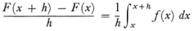
and using the mean value theorem for integrals Cauchy proves that
F′(x) = f(x).
This is the fundamental theorem of the calculus, and Cauchy’s presentation is the first demonstration of it. Then, after showing that all primitives of a given f(x) differ by a constant he defines the indefinite integral as
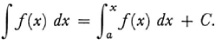
He points out that
presupposes f′(x) continuous. Cauchy then treats the singular (improper) integrals where f(x) becomes infinite at some value of x in the interval of integration or where the interval of integration extends to ∞. For the case where f(x) has a discontinuity at x = c at which value f(x) may be bounded or not Cauchy defines
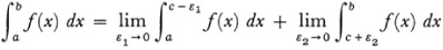
when these limits exist. When ε1 = ε2 we get what Cauchy called the principal value.
The notions of area bounded by a curve, length of a curve, volume bounded by surfaces and areas of surfaces had been accepted as intuitively understood, and it had been considered one of the great achievements of the calculus that these quantities could be calculated by means of integrals. But Cauchy, in keeping with his goal of arithmetizing analysis, defined these geometric quantities by means of the integrals which had been formulated to calculate them. Cauchy unwittingly imposed a limitation on the concepts he defined because the calculus formulas impose restrictions on the quantities involved. Thus the formula for the length of arc of a curve given by y = f(x) is
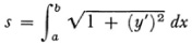
and this formula presupposes the differentiability of f(x) The question of what are the most general definitions of areas, lengths of curves, and volumes was to be raised later (Chap. 42, sec. 5).
Cauchy had proved the existence of an integral for any continuous integrand. He had also defined the integral when the integrand has jump discontinuities and infinities. But with the growth of analysis the need to consider integrals of more irregularly behaving functions became manifest. The subject of integrability was taken up by Riemann in his paper of 1854 on trigonometric series. He says that it is important at least for mathematics, though not for physical applications, to consider the broader conditions under which the integral formula for the Fourier coefficients holds.
Riemann generalized the integral to cover functions f(x) defined and bounded over an interval [a, b]. He breaks up this interval into subintervals26 Δx1, Δx2, …, Δxn and defines the oscillation of f(x) in Δxi as the difference between the greatest and least value of f(x) in Δxi. Then he proves that a necessary and sufficient condition that the sums
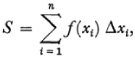
where xi is any value of x in Δxi approach a unique limit (that the integral exists) as the maximum Δxi approaches zero is that the sum of the intervals Δxi in which the oscillation of f(x) is greater than any given number λ must approach zero with the size of the intervals.
Riemann then points out that this condition on the oscillations allows him to replace continuous functions by functions with isolated discontinuities and also by functions having an everywhere dense set of points of discontinuity. In fact the example he gave of an integrable function with an infinite number of discontinuities in every arbitrarily small interval (sec. 3) was offered to illustrate the generality of his integral concept. Thus Riemann dispensed with continuity and piecewise continuity in the definition of the integral.
In his 1854 paper Riemann with no further remarks gives another necessary and sufficient condition that a bounded function f(x) be integrable on [a, b]. It amounts to first setting up what are now called the upper and lower sums
S = M1 Δx1 + … Mn Δxn
s = m1 Δx1 + … mn Δxn
where mi and Mi are the least and greatest values of f(x) in Δxi. Then letting Di = Mi – mi, Riemann states that the integral of f(x) over [a, b] exists if and only if

for all choices of Δxi filling out the interval [a, b]. Darboux completed this formulation and proved that the condition is necessary and sufficient.27 There are many values of S each corresponding to a partition of [a, b] into Δxi. Likewise there are many values of s. Each S is called an upper sum and each s a lower sum. Let the greatest lower bound of the S be J and the least upper bound of the s be I. It follows that I ≤ J. Darboux’s theorem then states that the sums S and s tend respectively to J and I when the number of Δxi is increased indefinitely in such a way that the maximum subinterval approaches zero. A bounded function is said to be integrable on [a, b] if J = I.
Darboux then shows that a bounded function will be integrable on [a, b] if and only if the discontinuities in f(x) constitute a set of measure zero. By the latter he meant that the points of discontinuity can be enclosed in a finite set of intervals whose total length is arbitrarily small. This very formulation of the integrability condition was given by a number of other men in the same year (1875). The terms upper integral and the notation  for the greatest lower bound J of the S’s, and lower integral and the notation
  for the least upper bound I of the s’s were introduced by Volterra.28
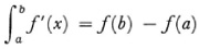
Darboux also showed in the 1875 paper that the fundamental theorem of the calculus holds for functions integrable in the extended sense. Bonnet had given a proof of the mean value theorem of the differential calculus which did not use the continuity of f′(x).29 Darboux using this proof, which is now standard, showed that
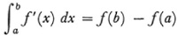
when f′ is merely integrable in the Riemann-Darboux sense. Darboux’s argument was that
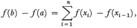
where a = x0 < x1 < x2 < … < xn = b. By the mean value theorem
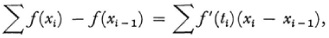
where ti is some value in (xi –1, xi). Now if the maximum Δxi, or xi – xi - 1 approaches zero then the right side of this last equation approaches  and the left side is f(b) – f(a).
One of the favorite activities of the 1870s and the 1880s was to construct functions with various infinite sets of discontinuities that would still be integrable in Riemann’s sense. In this connection H. J. S. Smith30 gave the first example of a function nonintegrable in Riemann’s sense but for which the points of discontinuity were “rare.” Dirichlet’s function (sec. 2) is also nonintegrable in this sense, but it is discontinuous everywhere.
The notion of integration was then extended to unbounded functions and to various improper integrals. The most significant extension was made in the next century by Lebesgue (Chap. 44). However, as far as the elementary calculus was concerned the notion of integral was by 1875 sufficiently broad and rigorously founded.
The theory of double integrals was also tackled. The simpler cases had been treated in the eighteenth century (Chap. 19, sec. 6). In his paper of 1814 (Chap. 27, sec. 4) Cauchy showed that the order of integration in which one evaluates a double integral ∫∫ f(x, y) dx dy does matter if the integrand is discontinuous in the domain of integration. Specifically Cauchy pointed out31 that the repeated integrals
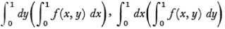
need not be equal when f is unbounded.
Karl J. Thomae (1840-1921) extended Riemann’s theory of integration to functions of two variables.32 Then Thomae in 187833 gave a simple example of a bounded function for which the second repeated integral exists but the first is meaningless.
In the examples of Cauchy and Thomae the double integral does not exist. But in 188334 Du Bois-Reymond showed that even when the double integral exists the two repeated integrals need not. In the case of double integrals too the most significant generalization was made by Lebesgue.
The eighteenth-century mathematicians used series indiscriminately. By the end of the century some doubtful or plainly absurd results from work with infinite series stimulated inquiries into the validity of operations with them. Around 1810 Fourier, Gauss, and Bolzano began the exact handling of infinite series. Bolzano stressed that one must consider convergence and criticized in particular the loose proof of the binomial theorem. Abel was the most outspoken critic of the older uses of series.
In his 1811 paper and his Analytical Theory of Heat Fourier gave a satisfactory definition of convergence of an infinite series, though in general he worked freely with divergent series. In the book (p. 196 of the English edition) he describes convergence to mean that as n increases the sum of n terms approaches a fixed value more and more closely and should differ from it only by a quantity which becomes less than any given magnitude. Moreover, he recognized that convergence of a series of functions may obtain only in an interval of x values. He also stressed that a necessary condition for convergence is that the terms approach zero in value. However, the series 1 – 1 + 1 + … still fooled him; he took its sum to be 1/2.
The first important and strictly rigorous investigation of convergence was made by Gauss in his 1812 paper “Disquisitiones Generales Circa Seriem Infinitam” (General Investigations of Infinite Series)35 wherein he studied the hypergeometric series F (α, β, γ, δ). In most of his work he called a series convergent if the terms from a certain one on decrease to zero. But in his 1812 paper he noted that this is not the correct concept. Because the hypergeometric series can represent many functions for different choices of α, β, and γ it seemed desirable to him to develop an exact criterion for convergence for this series. The criterion is laboriously arrived at but it does settle the question of convergence for the cases it was designed to cover. He showed that the hypergeometric series converges for real and complex x if |x| < 1 and diverges if |x| > 1. For x = 1, the series converges if and only if α + β < γ and for x = – 1 the series converges if and only if α + β < γ + 1. The unusual rigor discouraged interest in the paper by mathematicians of the time. Moreover, Gauss was concerned with particular series and did not take up general principles of the convergence of series.
Though Gauss is often mentioned as one of the first to recognize the need to restrict the use of series to their domains of convergence he avoided any decisive position. He was so much concerned to solve concrete problems by numerical calculation that he used Stirling’s divergent development of the gamma function. When he did investigate the convergence of the hypergeometric series in 1812 he remarked36 that he did so to please those who favored the rigor of the ancient geometers, but he did not state his own stand on the subject. In the course of his paper37 he used the development of log (2 – 2 cos x) in cosines of multiples of x even though there was no proof of the convergence of this series and there could have been no proof with the techniques available at the time. In his astronomical and geodetic work Gauss, like the eighteenth-century men, followed the practice of using a finite number of terms of an infinite series and neglecting the rest. He stopped including terms when he saw that the succeeding terms were numerically small and of course did not estimate the error.
Poisson too took a peculiar position. He rejected divergent series38 and even gave examples of how reckoning with divergent series can lead to false results. But he nevertheless made extensive use of divergent series in his representation of arbitrary functions by series of trigonometric and spherical functions.
Bolzano in his 1817 publication had the correct notion of the condition for the convergence of a sequence, the condition now ascribed to Cauchy. Bolzano also had clear and correct notions about the convergence of series. But, as we have already noted, his work did not become widely known.
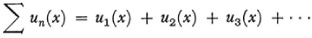
Cauchy’s work on the convergence of series is the first extensive significant treatment of the subject. In his Cours d’analyse Cauchy says, “Let
sn = u0 + u1 + … + un - 1
be the sum of the first n terms [of the infinite series which one considers], n designating a natural number. If, for constantly increasing values of n, the sum sn approaches indefinitely a certain limit s, the series will be called convergent, and the limit in question will be called the sum of the series.39 On the contrary, if while n increases indefinitely, the sum sn does not approach a fixed limit, the series will be called divergent and will have no sum.”
After defining convergence and divergence Cauchy states (Cours, p. 125) the Cauchy convergence criterion, namely, a sequence {Sn} converges to a limit S if and only if, Sn+r – Sn can be made less in absolute value than any assignable quantity for all r and sufficiently large n. Cauchy proves this condition is necessary but merely remarks that if the condition is fulfilled, the convergence of the sequence is assured. He lacked the knowledge of properties of real numbers to make the proof.
Cauchy then states and proves specific tests for the convergence of series with positive terms. He points out that un must approach zero. Another test (Cours, 132-35) requires that one find the limit or limits toward which the expression (un)1/n tends as n becomes infinite, and designate the greatest of these limits by k. Then the series will be convergent if k < 1 and divergent if k > 1. He also gives the ratio test which uses limn→∞ un + 1/un. If this limit is less than 1 the series converges and if greater than 1, the series diverges. Special tests are given if the ratio is 1. There follow comparison tests and a logarithmic test. He proves that the sum un + vn of two convergent series converges to the sum of the separate sums and the analogous result for product. Series with some negative terms, Cauchy shows, converge when the series of absolute values of the terms converge, and he then deduces Leibniz’s test for alternating series.
Cauchy also considered the sum of a series
in which all the terms are continuous, single-valued real functions. The theorems on the convergence of series of constant terms apply here to determine an interval of convergence. He also considers series with complex functions as terms.
Lagrange was the first to state Taylor’s theorem with a remainder but Cauchy in his 1823 and 1829 texts made the important point that the infinite Taylor series converges to the function from which it is derived if the remainder approaches zero. He gives the example 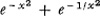 of a function whose Taylor series does not converge to the function. In his 1823 text he gives the example
  of a function which has all derivatives at x = 0 but has no Taylor expansion around x = 0. Here he contradicts by an example Lagrange’s assertion in his Théorie des fonctions (Ch. V., Art. 30) that if f(x) has at x0 all derivatives then it can be expressed as a Taylor series which converges to f(x) for x near x0. Cauchy also gave40 an alternative form for the remainder in Taylor’s formula.
Cauchy here made some additional missteps with respect to rigor. In his Cours d’analyse (pp. 131-32) he states that F(x) is continuous if when 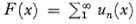 the series is convergent and the un(x) are continuous. In his Résumé des leçons41 he says that if the un(x) are continuous and the series converges then one may integrate the series term by term; that is,
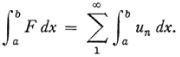
He overlooked the need for uniform convergence. He also asserts for continuous functions42 that
Cauchy’s work inspired Abel. Writing to his former teacher Holmboë from Paris in 1826 Abel said43 Cauchy “is at present the one who knows how mathematics should be treated.” In that year44 Abel investigated the domain of convergence of the binomial series

with m and x complex. He expressed astonishment that no one had previously investigated the convergence of this most important series. He proves first that if the series

wherein the vi’s are constants and α is real, converges for a value δ of α then it will converge for every smaller value of α, and f(α – β) for β approaching 0 will approach f(α) when α is equal to or smaller than δ. The last part says that a convergent power series is a continuous function of its argument up to and including δ, for α can be δ.
In this same 1826 paper45 Abel corrected Cauchy’s error on the continuity of the sum of a convergent series of continuous functions. He gave the example of
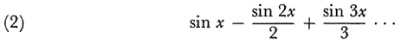
which is discontinuous when x = (2n + 1)π and n is integral, though the individual terms are continuous.46 Then by using the idea of uniform convergence he gave a correct proof that the sum of a uniformly convergent series of continuous functions is continuous in the interior of the interval of convergence. Abel did not isolate the property of uniform convergence of a series.
The notion of uniform convergence of a series  requires that given any ε, there exists an N such that for all n > N,
 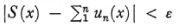 for all x in some interval. S(x) is of course the sum of the series. This notion was recognized in and for itself by Stokes, a leading mathematical physicist,47 and independently by Philipp L. Seidel (1821-96).48 Neither man gave the precise formulation. Rather both showed that if a sum of a series of continuous functions is discontinuous at x0 then there are values of x near x0 for which the series converges arbitrarily slowly. Also neither related the need for uniform convergence to the justification of integrating a series term by term. In fact, Stokes accepted49 Cauchy’s use of term-by-term integration. Cauchy ultimately recognized the need for uniform convergence50 in order to assert the continuity of the sum of a series of continuous functions but even he at that time did not see the error in his use of term-by-term integration of series.
Actually Weierstrass51 had the notion of uniform convergence as early as 1842. In a theorem that duplicates unknowingly Cauchy’s theorem on the existence of power series solutions of a system of first order ordinary differential equations, he affirms that the series converge uniformly and so constitute analytic functions of the complex variable. At about the same time Weierstrass used the notion of uniform convergence to give conditions for the integration of a series term by term and conditions for differentiation under the integral sign.
Through Weierstrass’s circle of students the importance of uniform convergence was made known. Heine emphasized the notion in a paper on trigonometric series.52 Heine may have learned of the idea through Georg Cantor who had studied at Berlin and then came to Halle in 1867 where Heine was a professor of mathematics.
During his years as a high-school teacher Weierstrass also discovered that any continuous function over a closed interval of the real axis can be expressed in that interval as an absolutely and uniformly convergent series of polynomials. Weierstrass included also functions of several variables. This result53 aroused considerable interest and many extensions of this result to the representation of complex functions by a series of polynomials or a series of rational functions were established in the last quarter of the nineteenth century.
It had been assumed that the terms of a series can be rearranged at will. In a paper of 1837 54 Dirichlet proved that in an absolutely convergent series one may group or rearrange terms and not change the sum. He also gave examples to show that the terms of any conditionally convergent series can be rearranged so that the sum is altered. Riemann in a paper written in 1854 (see below) proved that by suitable rearrangement of the terms the sum could be any given number. Many more criteria for the convergence of infinite series were developed by leading mathematicians from the 1830s on throughout the rest of the century.
As we know Fourier’s work showed that a wide class of functions can be represented by trigonometric series. The problem of finding precise conditions on the functions which would possess a convergent Fourier series remained open. Efforts by Cauchy and Poisson were fruitless.
Dirichlet took an interest in Fourier series after meeting Fourier in Paris during the years 1822-25. In a basic paper “Sur la convergence des séries trigonométriques”55 Dirichlet gave the first set of sufficient conditions that the Fourier series representing a given f(x) converge and converge to f(x). The proof given by Dirichlet is a refinement ofthat sketched by Fourier in the concluding sections of his Analytical Theory of Heat. Consider f(x) either given periodic with period 2π or given in the interval [–π, π] and defined to be periodic in each interval of length 2π to the left and right of [–π, π]. Dirichlet’s conditions are:
(a) f(x) is single-valued and bounded.
(b) f(x) is piecewise continuous; that is, it has only a finite number of discontinuities in the (closed) period.
(c) f(x) is piecewise monotone; that is, it has only a finite number of maxima and minima in one period.
The f(x) can have different analytic representations in different parts of the fundamental period.
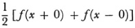
Dirichlet’s method of proof was to make a direct summation of n terms and to investigate what happens as n becomes infinite. He proved that for any given value of x the sum of the series is f(x) provided f(x) is continuous at that value of x and is (l/2)[f(x – 0) + f(x + 0)] if f(x) is discontinuous at that value of x.
In his proof Dirichlet had to give a careful discussion of the limiting values of the integrals
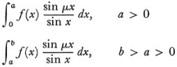
as μ increases indefinitely. These are still called the Dirichlet integrals.
It was in connection with this work that he gave the function which is c for rational values of x and d for irrational values of x (sec. 2). He had hoped to generalize the notion of integral so that a larger class of functions could still be representable by Fourier series converging to these functions, but the particular function just noted was intended as an example of one which could not be included in a broader notion of integral.
Riemann studied for a while under Dirichlet in Berlin and acquired an interest in Fourier series. In 1854 he took up the subject in his Habilitations-schrift (probationary essay) at Göttingen,56 “Über die Darstellbarkeit einer Function durch eine trigonometrische Reihe,” which aimed to find necessary and sufficient conditions that a function must satisfy so that at a point x in the interval [–π, π] the Fourier series for f(x) should converge to f(x).
Riemann did prove the fundamental theorem that if f(x) is bounded and integrable in [– π, π] then the Fourier coefficients

approach zero as n tends to infinity. The theorem showed too that for bounded and integrable f(x) the convergence of its Fourier series at a point in [– π, π] depends only on the behavior f(x) in the neighborhood of that point. However, the problem of finding necessary and sufficient conditions on f(x) so that its Fourier series converges to f(x) was not and has not been solved.
Riemann opened up another line of investigation. He considered trigonometric series but did not require that the coefficients be determined by the formula (3) for the Fourier coefficients. He starts with the series
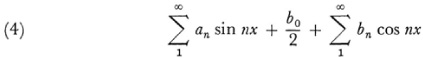
and defines
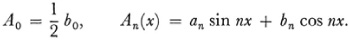
Then the series (4) is equal to
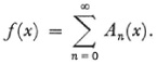
Of course f(x) has a value only for those values of x for which the series converges. Let us refer to the series itself by Ω. Now the terms of Ω may approach zero for all x or for some x. These two cases are treated separately by Riemann.
If an and bn approach zero, the terms of Ω approach zero for all x. Let F(x) be the function

which is obtained by two successive integrations of Ω. Riemann shows that F(x) converges for all x and is continuous in x. Then F(x) can itself be integrated. Riemann now proves a number of theorems about F(x) which lead in turn to necessary and sufficient conditions for a series of the form (4) to converge to a given function f(x) of period 2π. He then gives a necessary and sufficient condition that the trigonometric series (4) converge at a particular value of x, with an and bn still approaching 0 as n approaches ∞.
Next he considers the alternate case where limn → ∞ An depends on the value of x and gives conditions which hold when the series Ω is convergent for particular values of x and a criterion for convergence at particular values of x.
He also shows that a given f(x) may be integrable and yet not have a Fourier series representation. Further there are nonintegrable functions to which the series Ω converges for an infinite number of values of x taken between arbitrarily close limits. Finally a trigonometric series can converge for an infinite number of values of x in an arbitrarily small interval even though an and bn do not approach zero for all x.
The nature of the convergence of Fourier series received further attention after the introduction of the concept of uniform convergence by Stokes and Seidel. It had been known since Dirichlet’s time that the series were, in general, only conditionally convergent, if at all, and that their convergence depended upon the presence of positive and negative terms. Heine noted in a paper of 187057 that the usual proof that a bounded f(x) is uniquely represented between –π and π by a Fourier series is incomplete because the series may not be uniformly convergent and so cannot be integrated term by term. This suggested that there may nevertheless exist nonuniformly converging trigonometric series which do represent a function. Moreover, a continuous function might be representable by a Fourier series and yet the series might not be uniformly convergent. These problems gave rise to a new series of investigations seeking to establish the uniqueness of the representation of a function by a trigonometric series and whether the coefficients are necessarily the Fourier coefficients. Heine in the above-mentioned paper proved that a Fourier series which represents a bounded function satisfying the Dirichlet conditions is uniformly convergent in the portions of the interval [–π, π] which remain when arbitrarily small neighborhoods of the points of discontinuity of the function are removed from the interval. In these neighborhoods the convergence is necessarily nonuniform. Heine then proved that if the uniform convergence just specified holds for a trigonometric series which represents a function, then the series is unique.
The second result, on uniqueness, is equivalent to the statement that if a trigonometric series of the form
is uniformly convergent and represents zero where convergent, that is, except on a finite set P of points, then the coefficients are all zero and of course then the series represents zero throughout [–π, π].
The problems associated with the uniqueness of trigonometric and Fourier series attracted Georg Cantor, who studied Heine’s work. Cantor began his investigations by seeking uniqueness criteria for trigonometric series representations of functions. He proved58 that when f(x) is represented by a trigonometric series convergent for all x, there does not exist a different series of the same form which likewise converges for every x and represents the same f(x). Another paper59 gave a better proof for this last result.
The uniqueness theorem he proved can be restated thus: If, for all x, there is a convergent representation of zero by a trigonometric series, then the coefficients an and bn are zero. Then Cantor demonstrates in the 1871 paper that the conclusion still holds even if the convergence is renounced for a finite number of x values. This paper was the first of a sequence of papers in which Cantor treats the sets of exceptional values of x. He extended60 the uniqueness result to the case where an infinite set of exceptional values is permitted. To describe this set he first defined a point p to be a limit of a set of points S if every interval containing p contains infinitely many points of S. Then he introduced the notion of the derived set of a set of points. This derived set consists of the limit points of the original set. There is, then, a second derived set, that is, the derived set of the derived set, and so forth. If the nth derived set of a given set is a finite set of points then the given set is said to be of the nth kind or nth order (or of the first species). Cantor’s final answer to the question of whether a function can have two different trigonometric series representations in the interval [–π, π] or whether zero can have a non-zero Fourier representation is that if in the interval a trigonometric series adds up to zero for all x except those of a point set of the nth kind (at which one knows nothing more about the series) then all the coefficients of the series must be zero. In this 1872 paper Cantor laid the foundation of the theory of point sets which we shall consider in a later chapter. The problem of uniqueness was pursued by many other men in the last part of the nineteenth century and the early part of the twentieth.61
For about fifty years after Dirichlet’s work it was believed that the Fourier series of any function continuous in [–π π] converged to the function. But Du Bois-Reymond 62 gave an example of a function continuous in (–π, π) whose Fourier series did not converge at a particular point. He also constructed another continuous function whose Fourier series fails to converge at the points of an everywhere dense set. Then in 1875 63 he proved that if a trigonometric series of the form
converged to f(x) in [–π, π] and if f(x) is integrable (in a sense even more general than Riemann’s in that f(x) can be unbounded on a set of the first species) then the series must be the Fourier series for f(x). He also showed64 that any Fourier series of a function that is Riemann integrable can be integrated term by term even though the series is not uniformly convergent.
Many men then took up the problem already answered in one way by Dirichlet, namely, to give sufficient conditions that a function f(x) have a Fourier series which converges to f(x). Several results are classical. Jordan gave a sufficient condition in terms of the concept of a function of bounded variation, which he introduced.65 Let f(x) be bounded in [a, b] and let a = x0, x1, …, xn - 1, xn = b be a mode of division (partition) of this interval. Let y0, y1, …, yn - 1 be the values of f(x) at these points. Then, for every partition
let t denote
To every mode of subdividing [a, b] there is a t. When corresponding to all possible modes of division of [a, b], the sums t have a least upper bound then f is defined to be of bounded variation in [a, b].
Jordan’s sufficient condition states that the Fourier series for the integrable function f(x) converges to
at every point for which there is a neighborhood in which f (x) is of bounded variation.66
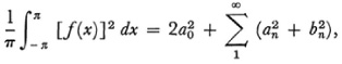
During the 1860s and 1870s the properties of the Fourier coefficients were also examined and among the important results obtained were what is called Parseval’s theorem (who stated it under more restricted conditions, Chap. 29, sec. 3) according to which if f(x) and [f(x)]2 are Riemann integrable in [–π, π] then
and if f(x) and g(x) and their squares are Riemann integrable then
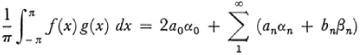
where an, bn, αn and βn are the Fourier coefficients of f(x) and g(x) respectively.
The work of Bolzano, Cauchy, Weierstrass, and others supplied the rigor in analysis. This work freed the calculus and its extensions from all dependence upon geometrical notions, motion, and intuitive understandings. From the outset these researches caused a considerable stir. After a scientific meeting at which Cauchy presented his theory on the convergence of series Laplace hastened home and remained there in seclusion until he had examined the series in his Mécanique céleste. Luckily every one was found to be convergent. When Weierstrass’s work became known through his lectures, the effect was even more noticeable. The improvements in rigor can be seen by comparing the first edition of Jordan’s Cours d’analyse (1882-87) with the second (189396) and the third edition (3 vols., 1909-15). Many other treatises incorporated the new rigor.
The rigorization of analysis did not prove to be the end of the investigation into the foundations. For one thing, practically all of the work presupposed the real number system but this subject remained unorganized. Except for Weierstrass who, as we shall see, considered the problem of the irrational number during the 1840s, all the others did not believe it necessary to investigate the logical foundations of the number system. It would appear that even the greatest mathematicians must develop their capacities to appreciate the need for rigor in stages. The work on the logical foundations of the real number system was to follow shortly (Chap. 41).
The discovery that continuous functions need not have derivatives, that discontinuous functions can be integrated, the new light on discontinuous functions shed by Dirichlet’s and Riemann’s work on Fourier series, and the study of the variety and the extent of the discontinuities of functions made the mathematicians realize that the rigorous study of functions extends beyond those used in the calculus and the usual branches of analysis where the requirement of differentiability usually restricts the class of functions. The study of functions was continued in the twentieth century and resulted in the development of a new branch of mathematics known as the theory of functions of a real variable (Chap. 44).
Like all new movements in mathematics, the rigorization of analysis did not go unopposed. There was much controversy as to whether the refinements in analysis should be pursued. The peculiar functions that were introduced were attacked as curiosities, nonsensical functions, funny functions, and as mathematical toys perhaps more intricate but of no more consequence than magic squares. They were also regarded as diseases or part of the morbid pathology of functions and as having no bearing on the important problems of pure and applied mathematics. These new functions, violating laws deemed perfect, were looked upon as signs of anarchy and chaos which mocked the order and harmony previous generations had sought. The many hypotheses which now had to be made in order to state a precise theorem were regarded as pedantic and destructive of the elegance of the eighteenth-century classical analysis, “as it was in paradise,” to use Du Bois-Reymond’s phrasing. The new details were resented as obscuring the main ideas.
Poincaré, in particular, distrusted this new research. He said:67
Logic sometimes makes monsters. For half a century we have seen a mass of bizarre functions which appear to be forced to resemble as little as possible honest functions which serve some purpose. More of continuity, or less of continuity, more derivatives, and so forth. Indeed from the point of view of logic, these strange functions are the most general; on the other hand those which one meets without searching for them, and which follow simple laws appear as a particular case which does not amount to more than a small corner.
In former times when one invented a new function it was for a practical purpose; today one invents them purposely to show up defects in the reasoning of our fathers and one will deduce from them only that.
Charles Hermite said in a letter to Stieltjes, “I turn away with fright and horror from this lamentable evil of functions which do not have derivatives.”
Another kind of objection was voiced by Du Bois-Reymond.68 His concern was that the arithmetization of analysis separated analysis from geometry and consequently from intuition and physical thinking. It reduced analysis “to a simple game of symbols where the written signs take on the arbitrary significance of the pieces in a chess or card game.”
The issue that provoked the most controversy was the banishment of divergent series notably by Abel and Cauchy. In a letter to Holmboë, written in 1826, Abel says,69
The divergent series are the invention of the devil, and it is a shame to base on them any demonstration whatsoever. By using them, one may draw any conclusion he pleases and that is why these series have produced so many fallacies and so many paradoxes. … I have become prodigiously attentive to all this, for with the exception of the geometrical series, there does not exist in all of mathematics a single infinite series the sum of which has been determined rigorously. In other words, the things which are most important in mathematics are also those which have the least foundation.
However, Abel showed some concern about whether a good idea had been overlooked because he continues his letter thus: “That most of these things are correct in spite of that is extraordinarily surprising. I am trying to find a reason for this; it is an exceedingly interesting question.” Abel died young and so never did pursue the matter.
Cauchy, too, had some qualms about ostracizing divergent series. He says in the introduction of his Cours (1821), “I have been forced to admit diverse propositions which appear somewhat deplorable, for example, that a divergent series cannot be summed.” Despite this conclusion Cauchy continued to use divergent series as in notes appended to the publication in 182770 of a prize paper written in 1815 on water waves. He decided to look into the question of why divergent series proved so useful and as a matter of fact he ultimately did come close to recognizing the reason (Chap. 47).
The French mathematicians accepted Cauchy’s banishment of divergent series. But the English and the Germans did not. In England the Cambridge school defended the use of divergent series by appealing to the principle of permanence of form (Chap. 32, sec. 1). In connection with divergent series the principle was first used by Robert Woodhouse (1773-1827). In The Principles of Analytic Calculation (1803, p. 3) he points out that in the equation
the equality sign has “a more extended signification” than just numerical equality. Hence the equation holds whether the series diverges or not.
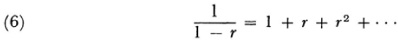
Peacock, too, applied the principle of permanence of forms to operations with divergent series.71 On page 267 he says, “Thus since for r < 1, (6) above holds, then for r = 1 we do get ∞ = 1 + 1 + 1 + …. For r > 1 we get a negative number on the left and, because the terms on the right continually increase, a quantity more than ∞ on the right.” This Peacock accepts. The point he tries to make is that the series can represent 1/(1 – r) for all r. He says,
If the operations of algebra be considered as general, and the symbols which are subject to them as unlimited in value, it will be impossible to avoid the formation of divergent as well as convergent series; and if such series be considered as the results of operations which are definable, apart from the series themselves, then it will not be very important to enter into such an examination of the relation of the arithmetical values of the successive terms as may be necessary to ascertain their convergence or divergence; for under such circumstances, they must be considered as equivalent forms representing their generating function, and as possessing for the purposes of such operations, equivalent properties. … The attempt to exclude the use of divergent series in symbolical operations would necessarily impose a limit upon the universality of algebraic formulas and operations which is altogether contrary to the spirit of science. … It would necessarily lead to a great and embarrassing multiplication of cases: it would deprive almost all algebraical operations of much of their certainty and simplicity.
Augustus De Morgan, though much sharper and more aware than Peacock of the difficulties in divergent series, was nevertheless under the influence of the English school and also impressed by the results obtained by the use of divergent series despite the difficulties in them. In 1844 he began an acute and yet confused paper on “Divergent Series”72 with these words, “I believe it will be generally admitted that the heading of this paper describes the only subject yet remaining, of an elementary character, on which a serious schism exists among mathematicians as to absolute correctness or incorrectness of results.” The position De Morgan took he had already declared in his Differential and Integral Calculus:73 “The history of algebra shows us that nothing is more unsound than the rejection of any method which naturally arises, on account of one or more apparently valid cases in which such a method leads to erroneous results. Such cases should indeed teach caution, but not rejection; if the latter had been preferred to the former, negative quantities, and still more their square roots, would have been an effectual bar to the progress of algebra … and those immense fields of analysis over which even the rejectors of divergent series now range without fear, would have been not so much as discovered, much less cultivated and settled. … The motto which I should adopt against a course which seems to me calculated to stop the progress of discovery would be contained in a word and a symbol—remember  .” He distinguishes between the arithmetic and algebraic significance of a series. The algebraic significance holds in all cases. To account for some of the false conclusions obtained with divergent series he says in the 1844 paper (p. 187) that integration is an arithmetic and not an algebraic operation and so could not be applied without further thought to divergent series. But the derivation of
by starting with y = 1 + ry, replacing y on the right by 1 + ry, and continuing thus, he accepts because it is algebraic. Likewise from z = 1 + 2z one gets z = 1 + 2 + 4 + …. Hence –1 = 1 + 2 + 4 + … and this is right. He accepts the entire theory (as of that date) of trigonometric series but would be willing to reject it if one could give one instance where 1 – 1 + 1 – 1 + … does not equal 1/2 (see Chap. 20).
Many other prominent English mathematicians gave other kinds of justification for the acceptance of divergent series, some going back to an argument of Nicholas Bernoulli (Chap. 20, sec. 7) that the series (6) contains a remainder r∞ or r∞/(1 – r∞). This must be taken into account (though they did not indicate how). Others said the sum of a divergent series is algebraically true but arithmetically false.
Some German mathematicians used the same arguments as Peacock though they used different words, such as syntactical operations as opposed to arithmetical operations or literal as opposed to numerical. Martin Ohm74 said, “An infinite series (leaving aside any question of convergence or divergence) is completely suited to represent a given expression if one can be sure of having the correct law of development of the series. Of the value of an infinite series one can speak only if it converges.” Arguments in Germany in favor of the legitimacy of divergent series were advanced for several more decades.
The defense of the use of divergent series was not nearly so foolish as it might seem, though many of the arguments given in behalf of the series were, perhaps, far-fetched. For one thing in the whole of eighteenth-century analysis the attention to rigor or proof was minimal and this was acceptable because the results obtained were almost always correct. Hence mathematicians became accustomed to loose procedures and arguments. But, even more to the point, many of the concepts and operations which had caused perplexities, such as complex numbers, were shown to be correct after they were fully understood. Hence mathematicians thought that the difficulties with divergent series would also be cleared up when a better understanding was obtained and that divergent series would prove to be legitimate. Further the operations with divergent series were often bound up with other little understood operations of analysis such as the interchange of the order of limits, integration over discontinuities of an integrand and integration over an infinite interval, so that the defenders of divergent series could maintain that the false conclusions attributed to the use of divergent series came from other sources of trouble.
One argument which might have been brought up is that when an analytic function is expressed in some domain by a power series, what Weierstrass called an element, this series does indeed carry with it the “algebraic” or “syntactical” properties of the function and these properties are carried beyond the domain of convergence of the element. The process of analytic continuation uses this fact. Actually there was sound mathematical substance in the concept of divergent series which accounted for their usefulness. But the recognition of this substance and the final acceptance of divergent series had to await a new theory of infinite series (Chap. 47).
Abel, N. H.: Œuvres complètes, 2 vols., 1881, Johnson Reprint Corp., 1964.
——: Mémorial publié à l’occasion du centenaire de sa naissance, Jacob Dybwad, 1902. Letters to and from Abel.
Bolzano, B.: Rein analytischer Beweis des Lehrsatzes, dass zwischen je zwei Werthen, die ein entgegengesetztes Resultat gewähren, wenigstens eine reele Wurzel der Gleichung liege, Gottlieb Hass, Prague, 1817 = Abh. Königl. Böhm. Ges. der Wiss., (3), 5, 1814-17, pub. 1818 = Ostwald’s Klassiker der exakten Wissenschaften #153, 1905, 3-43. Not contained in Bolzano’s Schriften.
——: Paradoxes of the Infinite, Routledge and Kegan Paul, 1950. Contains a historical survey of Bolzano’s work.
——: Schriften, 5 vols., Königlichen Böhmischen Gesellschaft der Wissenschaften, 1930-48.
Boyer, Carl B.: The Concepts of the Calculus, Dover (reprint), 1949, Chap. 7.
Burkhardt, H.: “Über den Gebrauch divergenter Reihen in der Zeit von 1750-1860,” Math. Ann., 70, 1911, 169-206.
——: “Trigonometrische Reihe und Integrale,” Encyk. der Math. Wiss., II A12, 819-1354, B. G. Teubner, 1904-16.
Cantor, Georg: Gesammelte Abhandlungen (1932), Georg Olms (reprint), 1962.
Cauchy, A. L.: Œuvres, (2), Gauthier-Villars, 1897-99, Vols. 3 and 4.
Dauben, J. W.: “The Trigonometrie Background to Georg Cantor’s Theory of Sets,” Archive for History of Exact Sciences, 7, 1971, 181-216.
Dirichlet, P. G. L.: Werke, 2 vols. Georg Reimer, 1889-97, Chelsea (reprint), 1969.
Du Bois-Reymond, Paul: Zwei Abhandlungen über unendliche und trigonometrische Reihen (1871 and 1874), Ostwald’s Klassiker #185; Wilhelm Engelmann, 1913.
Freudenthal, H.: “Did Cauchy Plagiarize Bolzano?,” Archive for History of Exact Sciences, 7, 1971, 375-92.
Gibson, G. A.: “On the History of Fourier Series,” Proc. Edinburgh Math. Soc, 11, 1892/93, 137-66.
Grattan-Guinness, I.: “Bolzano, Cauchy and the ’New Analysis’ of the Nineteenth Century,” Archive for History of Exact Sciences, 6, 1970, 372-400.
—: The Development of the Foundations of Mathematical Analysis from Euler to Riemann, Massachusetts Institute of Technology Press, 1970.
Hawkins, Thomas W., Jr.: Lebesgue’s Theory of Integration: Its Origins and Development, University of Wisconsin Press, 1970, Chaps. 1-3.
Manheim, Jerome H.: The Genesis of Point Set Topology, Macmillan, 1964, Chaps. 1-4.
Pesin, Ivan N.: Classical and Modern Integration Theories, Academic Press, 1970, Chap. 1.
Pringsheim, A.: “Irrationalzahlen und Konvergenz unendlichen Prozesse,” Encyk. der Math. Wiss., IA3, 47-147, B. G. Teubner, 1898-1904.
Reiff, R.: Geschichte der unendlichen Reihen, H. Lauppsche Buchhandlung, 1889; Martin Sandig (reprint), 1969.
Riemann, Bernhard: Gesammelte mathematische Werke, 2nd. ed. (1902), Dover (reprint), 1953.
Schlesinger, L.: “Über Gauss’ Arbeiten zur Funktionenlehre,” Nachrichten König. Ges. der Wiss. zu Gött., 1912, Beiheft, 1-43. Also in Gauss’s Werke, 102, 77 ff.
Schoenflies, Arthur M.: “Die Entwicklung der Lehre von den Punktmannig-faltigkeiten,” Jahres, der Deut. Math.-Verein., 82, 1899, 1-250.
Singh, A. N.: “The Theory and Construction of Non-Differentiable Functions,” in E. W. Hobson: Squaring the Circle and Other Monographs, Chelsea (reprint), 1953.
Smith, David E.: A Source Book in Mathematics, Dover (reprint), 1959, Vol. 1,
286-91, Vol. 2, 635-37.
Stolz, O.: “B. Bolzanos Bedeutung in der Geschichte der Infinitesimalrechnung,” Math. Ann., 18, 1881, 255-79.
Weierstrass, Karl: Mathematische Werke, 7 vols., Mayer und Müller, 1894-1927.
Young, Grace C: “On Infinite Derivatives,” Quart. Jour, of Math., 47, 1916, 127-75.