Nature is not embarrassed by difficulties of analysis.
AUGUSTIN FRESNEL
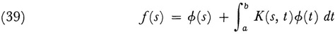
An integral equation is an equation in which an unknown function appears under an integral sign and the problem of solving the equation is to determine that function. As we shall soon see, some problems of mathematical physics lead directly to integral equations, and other problems, which lead first to ordinary or partial differential equations, can be handled more expeditiously by converting them to integral equations. At first, solving integral equations was described as inverting integrals. The term integral equations is due to Du Bois-Reymond.1
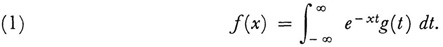
As in other branches of mathematics, isolated problems involving integral equations occurred long before the subject acquired a distinct status and methodology. Thus Laplace in 17822 considered the integral equation for g(t) given by
As equation (1) now stands, it is called the Laplace transform of g(t). Poisson3 discovered the expression for g(t), namely,
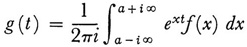
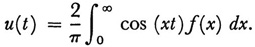
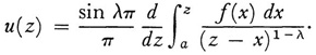
for large enough a. Another of the noteworthy results that really belong to the history of integral equations stems from Fourier’s famous 1811 paper on the theory of heat (Chap. 28, sec. 3). Here one finds
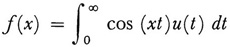
and the inversion formula
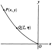
The first conscious direct use and solution of an integral equation go back to Abel. In two of his earliest published papers, the first published in an obscure journal in 18234 and the second published in the Journal für Mathematik,5 Abel considered the following mechanics problem: A particle starting at P slides down a smooth curve (Fig. 45.1) to the point 0. The curve lies in a vertical plane. The velocity acquired at 0 is independent of the shape of the curve but the time required to slide from P to O is not. If (ξ, η) are the coordinates of any point Q between s and 0 and s is the arc OQ, then the velocity of the particle at Q is given by
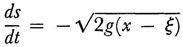
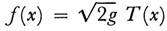
where g is the gravitational constant. Hence
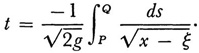
Now s can be expressed in terms of ξ. Suppose s is v (ξ). Then the whole time of descent T from P to O is given by
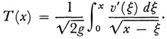
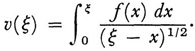
The time T clearly depends upon x for any curve. The problem Abel set was, given T as a function of x, to find v (ξ). If we introduce
the problem becomes to determine v from the equation
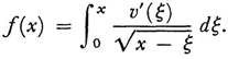
Abel obtained the solution
His methods—he gave two—were special and not worth noting.
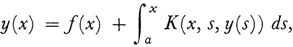
Actually Abel undertook to solve the more general problem
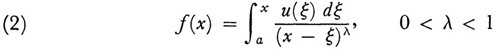
and obtained
Liouville, who worked independently of Abel, solved special integral equations from 1832 on.6 A more significant step by Liouville7 was to show how the solution of certain differential equations can be obtained by solving integral equations. The differential equation to be solved is

over the interval a ≤ x ≤ p is a parameter. Let u(x) be the particular solution that satisfies the initial conditions

This function will also be a solution of the nonhomogeneous equation
yn + ρ2y = σ(x)u(x).
Then by a basic result on ordinary differential equations,

Thus if we can solve this integral equation we shall have obtained that solution of the differential equation (3) that satisfies the initial conditions (4).
Liouville obtained the solution by a method of successive substitutions attributed to Carl G. Neumann, whose work Untersuchungen über das logarithmische und Newton’sehe Potential (1877) came thirty years later. We shall not describe Liouville’s method because it is practically identical with the one given by Volterra, which is to be described shortly.
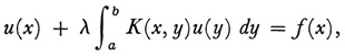
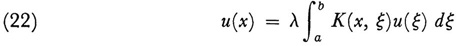
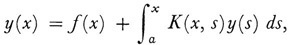
The integral equations treated by Abel and Liouville are of basic types. Abel’s is of the form
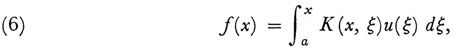
and Liouville’s of the form

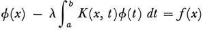
In both of these f(x) and K(x, ξ) are known, and u(ξ) is the function to be determined. The terminology used today, introduced by Hilbert, refers to these equations as the first and second kind, respectively, and K(x, ξ) is called the kernel. As stated, they are also referred to as Volterra’s equations, whereas when the upper limit is a fixed number b, they are called Fredholm’s equations. Actually the Volterra equations are special cases, respectively, of Fredholm’s because one can always take K(x, ξ) = 0 for ξ > x and then regard the Volterra equations as Fredholm equations. The special case of the equation of the second kind in which f(x) ≡ 0 is called the homogeneous equation.
By the middle of the nineteenth century the chief interest in integral equations centered around the solution of the boundary-value problem associated with the potential equation

The equation holds in a given plane area that is bounded by some curve C. If the boundary value of u is some function f(s) given as a function of arc length s along C, then a solution of this potential problem can be represented
by
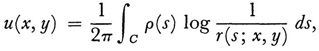
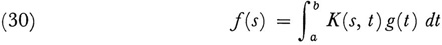
wherein r(s; x, y) is the distance from a point s to any point (x, y) in the interior or boundary and p(s) is an unknown function satisfying for s = (x, y) on C
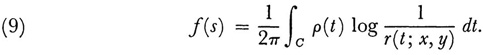
This is an integral equation of the first kind for p(t). Alternatively, if one takes as a solution of (8) with the same boundary condition
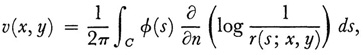
where ∂/∂n denotes the normal derivative to the boundary, then φ(s) must satisfy the integral equation

an integral equation of the second kind. These equations were solved by Neumann for convex areas in his Untersuchungen and later publications.
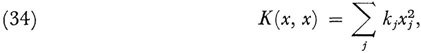
Another problem of partial differential equations was tackled through integral equations. The equation

arises in the study of wave motion when the time dependence of the corresponding hyperbolic equation
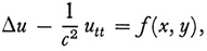
usually taken to be e-iωt, is eliminated. It was known (Chap. 28, sec. 8) that the homogeneous case of (11) subject to boundary conditions has nontrivial solutions only for a discrete set of λ-values, called eigenvalues or characteristic values. Poincaré in 18948 considered the inhomogeneous case (11) with complex λ. He was able to produce a function, meromorphic in λ, which represented a unique solution of (11) for any λ which is not an eigenvalue, and whose residues produce eigenfunctions for the homogeneous case, that is, when f = 0.
On the basis of these results, Poincaré in 18969 considered the equation
which he derived from (11), and affirmed that the solution is a meromorphic function of λ. This result was established by Fredholm in a paper we shall consider shortly.
The conversion of differential equations to integral equations, which is illustrated by the above examples, became a major technique for solving initial- and boundary-value problems of ordinary and partial differential equations and was the strongest impetus for the study of integral equations.
Vito Volterra (1860-1940), who succeeded Beltrami as professor of mathematical physics at Rome, is the first of the founders of a general theory of
integral equations. He wrote papers on the subject from 1884 on and principal ones in 1896 and 1897.10 Volterra contributed a method of solving integral equations of the second kind,
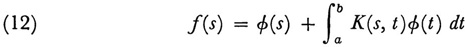
wherein φ(s) is unknown and K(s, t) = 0 for t > s. Volterra wrote this equation as
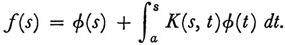
His method of solution was to let
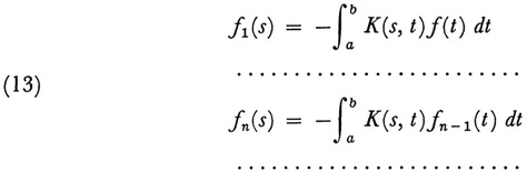
and take φ(s) to be
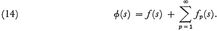
For his kernel K(s, t) Volterra was able to prove the convergence of (14), and if one substitutes (14) in (12), one can show that it is a solution. This substitution gives

which can be written in the form

where the kernel  (later called the solving kernel or resolvent by Hilbert) is
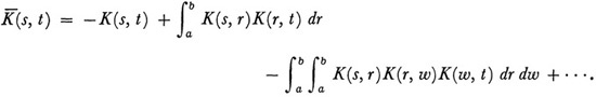
Equation (15) is the representation obtained earlier for a particular integral equation by Liouville and credited to Neumann. Volterra also solved integral equations of the first kind 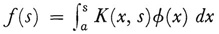 by reducing them to equations of the second kind.
In 1896 Volterra observed that an integral equation of the first kind is a limiting form of a system of n linear algebraic equations in n unknowns as n becomes infinite. Erik Ivar Fredholm (1866-1927), professor of mathematics at Stockholm, concerned with solving the Dirichlet problem, took up this idea in 190011 and used it to solve integral equations of the second kind, that is, equations of the form (12), without, however, the restriction on K(s, t).
We shall write the equation Fredholm tackled in the form

though the parameter λ was not explicit in his work. However, what he did is more intelligible in the light of later work if we exhibit it. To be faithful to Fredholm’s formulas, one should set λ = 1 or regard it as implicitly involved in K.
Fredholm divided the x-interval [a, b] into n equal parts by the points
a, x1 = a + δ, x2 = a + 2δ,…, xn = a + nδ = b.
He then replaced the definite integral in (16) by the sum
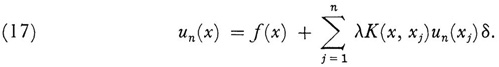
Now equation (17) is supposed to hold for all values of x in [a, b]. Hence it should hold for x = x1, x2,…, xn. This gives the system of n equations
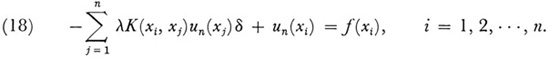
This system is a set of n nonhomogeneous linear equations for determining the n unknowns un(x1), un(x2),…, un(xn).
In the theory of linear equations the following result was known: If the matrix
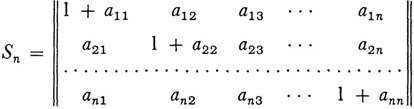
then the determinant D(n) of Sn has the following expansion:12
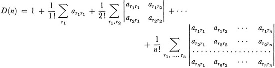
where r1; r2, . ., rn run independently over all the values from 1 to n. By expanding the determinant of the coefficients in (18), and then letting n become infinite, Fredholm obtained the determinant
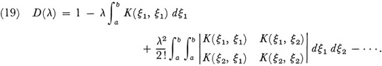
This he called the determinant of (16) or of the kernel K. Likewise, by considering the cofactor of the element in the vth row and μth column of the determinant of the coefficients in (18) and letting n become infinite, Fredholm obtained the function
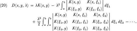
Fredholm called D(x, y, λ) the first minor of the kernel K because it plays the role analogous to first minors in the case of n linear equations in n unknowns. He also called the zeros of the integral analytic function D(λ) the roots of K(x, y). By applying Cramer’s rule to the system of linear equations (18) and by letting n become infinite, Fredholm inferred the form of the solution of (16). He then proved that it was correct by direct substitution and could assert the following results: If λ is not one of the roots of K, that is, if D(λ) ≠ 0, (16) has one and only one (continuous) solution, namely,

Fredholm obtained further results involving the relation between the homogeneous equation
and the inhomogeneous equation (16). It is almost evident from (21) that when λ is not a root of K the only continuous solution of (22) is u = 0. Hence he considered the case when λ is a root of K. Let λ = λ1 be such a root. Then (22) has the infinite number of solutions
c1u1(x) + c2u2(x)+ … + cnun(x),
where the  are arbitrary constants; the ul u2,…, un, called principal solutions, are linearly independent; and n depends upon λ1. The quantity n is called the index of λ1 [which is not the multiplicity of λ1 as a zero of D)(λ)]. Fredholm was able to determine the index of any root λi and to show that the index can never exceed the multiplicity (which is always finite). The roots of D(λ) = 0 are called the characteristic values of K(x, y) and the set of roots is called the spectrum. The solutions of (22) corresponding to the characteristic values are called eigenfunctions or characteristic functions.
And now Fredholm was able to establish what has since been called the Fredholm alternative theorem. In the case where A is a characteristic value of K not only does the integral equation (22) have n independent solutions but the associated or adjoint equation which has the transposed kernel, namely,
also has n solutions ψ1 (x),…, ψn(x) for the same characteristic value and then the nonhomogeneous equation (16) is solvable if and only if

These last few results parallel very closely the theory of a system of linear algebraic equations, homogeneous and nonhomogeneous.
A lecture by Erik Holmgren (b. 1872) in 1901 on Fredholm’s work on integral equations, which had already been published in Sweden, aroused Hilbert’s interest in the subject. David Hilbert (1862-1943), the leading mathematician of this century, who had already done superb work on algebraic numbers, algebraic invariants, and the foundations of geometry, now turned his attention to integral equations. He says that an investigation of the subject showed him that it was important for the theory of definite integrals, for the development of arbitrary functions in series (of special functions or trigonometric functions), for the theory of linear differential equations, for potential theory, and for the calculus of variations. He wrote a series of six papers from 1904 to 1910 in the Nachrichten von der Königlichen Gesellschaft der Wissenschaften zu Göttingen and reproduced these in his book Grundzüge einer allgemeinen Theorie der linearen Integralgleichungen(1912). During the latter part of this work he applied integral equations to problems of mathematical physics.
Fredholm had used the analogy between integral equations and linear algebraic equations, but instead of carrying out the limiting processes for the infinite number of algebraic equations, he boldly wrote down the resulting determinants and showed that they solved the integral equations. Hilbert’s first work was to carry out a rigorous passage to the limit on the finite system of linear equations.
He started with the integral equation

wherein K(s, t) is continuous. The parameter λ is explicit and plays a significant role in the subsequent theory. Like Fredholm, Hilbert divided up the interval [0, 1] into n parts so that p/n or q/n (p, q = 1, 2,…, n) denotes a coordinate in the interval [0, 1]. Let
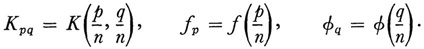
Then from (24) we obtain the system of n equations in n unknowns φ,…φn, namely,
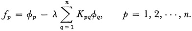
After reviewing the theory of solution of a finite system of n linear equations in n unknowns, Hilbert considers equation (24). For the kernel K(24) the eigenvalues are defined to be zeros of the power series
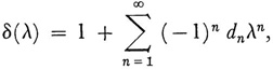
where the coefficients dn are given by
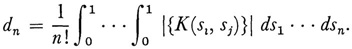
Here |{K(si, si)}| is the determinant of the n by n matrix |si, sj)}, i, j = 1, 2, …, n, amd the si are values of t in the interval [0, 1]. To indicate Hilbert’s major result we need the intermediate quantities
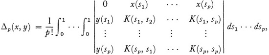
wherein x(r) and y(r) are arbitrary continuous functions of r on [0, 1], and
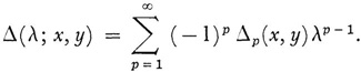
Hilbert next defines
Δ* (λ; s, t) = λΔ(λ;x, y) – δ(λ)
wherein now x(r) = K(s, r) and y(r) = K(r, t). He then proves that if is defined by
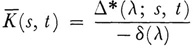
for values of λ for which δ(λ) ≠ 0, then
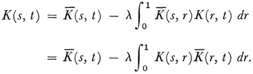
Finally if φ is taken to be

then φ is a solution of (24). The proofs of various steps in this theory involve a number of limit considerations on expressions which occur in Hubert’s treatment of the finite system of linear equations.
Thus far Hilbert showed that for any continuous (not necessarily symmetric) kernel K(s, t) and for any value of λ such that δ(λ) ≠ = 0, there exists the solving function (resolvent) (s, t), which has the property that (25) solves equation (24).
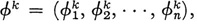
Now Hilbert assumes K(s, t) to be symmetric, which enables him to use facts about symmetric matrices in the finite case, and shows that the zeros of δ(λ), that is, the eigenvalues of the symmetric kernel, are real. Then the zeros of δ(λ) are ordered according to increasing absolute values (for equal absolute values the positive zero is taken first and any multiplicities are to be counted). The eigenfunctions of (24) are now defined by
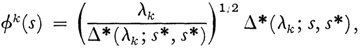
where s* is chosen so that Δ*(λk; s*, s*) ≠ 0 and λk is any eigenvalue of K (s, t).
The eigenfunctions associated with the separate eigenvalues can be chosen to be an orthonormal (orthogonal and normalized13) set and for each eigenvalue λk and for each eigenfunction belonging to λfc
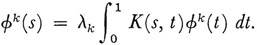
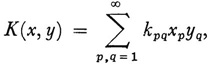
With these results Hilbert is able to prove what is called the generalized principal axis theorem for symmetric quadratic forms. First, let
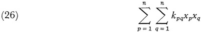
be an n-dimensional quadratic form in the n variables x1, x2,…xn, This can be written as (Kx, x) where K is the matrix of the kpq, x stands for the vector x1, x2,…xn and (Kx, x) is the inner product (scalar product) of the two vectors Kx and x. Suppose K has the n distinct eigenvalues λ1 λ2,…,…λ. Then for any fixed λk the equations
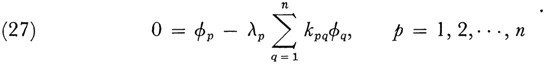
have the solution
which is a unique solution up to a constant multiple. It is then possible, as Hilbert showed, to write
wherein the parentheses again denote an inner product of vectors.
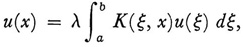
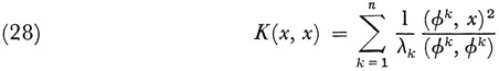
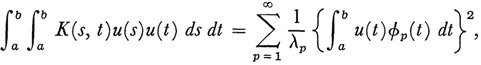
Hubert’s generalized principal axis theorem reads as follows: Let K(s, t) be a continuous symmetric function of s and t. Let φp(s) be the normalized eigenfunction belonging to the eigenvalue λp of the integral equation
(24). Then for arbitrary continuous x(s) and y(s), the following relation holds:

where α = n or ∞ depending on the number of eigenvalues and in the latter case the sum converges uniformly and absolutely for all x(s) and y(s) which satisfy
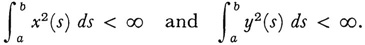
The generalization of (28) to (29) becomes apparent if we first define  as the inner product of any two functions u(s) and v(s) and denote it by (u, v). Now replace y(s) in (29) by x(s) and replace the left side of (28) by integration instead of summation.
Hilbert proved next a famous result, later called the Hilbert-Schmidt theorem. If f(s) is such that for some continuous g(s)
then
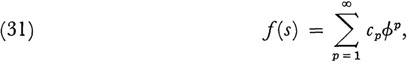
where the φv are the orthonormal eigenfunctions of K and
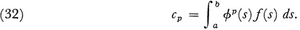
Thus an “arbitrary” function f(s) can be expressed as an infinite series in the eigenfunctions of K with coefficients cp that are the “ Fourier” coefficients of the expansion.
Hilbert, in the preceding work, had carried out limiting processes that generalized results on finite systems of linear equations and finite quadratic forms to integrals and integral equations. He decided that a treatment of infinite quadratic forms themselves, that is, quadratic forms with infinitely many variables, would “form an essential completion of the well-known theory of quadratic forms with finitely many variables.” He therefore took up what may be called purely algebraic questions. He considers the infinite bilinear form
and by passing to the limit of results for bilinear and quadratic forms in 2n and n variables respectively, obtains basic results. The details of the work are considerable and we shall only note some of the results. Hilbert first obtains an expression for a resolvent form (λ; x, x), which has the peculiar feature that it is the sum of expressions, one for each of a discrete set of values of λ, and of an integral over a set of λ belonging to a continuous range. The discrete set of λ values belongs to the point spectrum of K, and the continuous set to the continuous or band spectrum. This is the first significant use of continuous spectra, which had been observed for partial differential equations by Wilhelm Wirtinger (b. 1865) in 1896.14
To get at the key result for quadratic forms, Hilbert introduces the notion of a bounded form. The notation (x, x) denotes the inner (scalar) product of the vector (x1, x2, xn,…) with itself and (x, y) has the analogous meaning. Then the form K(x, y) is said to be bounded if |K(x, y) ≤ M for all x and y such that (x, x) ≤ 1 and (y, y) ≤ 1. Boundedness implies continuity, which Hilbert defines for a function of infinitely many variables.
Hubert’s key result is the generalization to quadratic forms in infinitely many variables of the more familiar principal axis theorem of analytic geometry. He proves that there exists an orthogonal transformation T such that in the new variables  where x’ = Tx, K can be reduced to a “sum of squares.” That is, every bounded quadratic form
  can be transformed by a unique orthogonal transformation into the form
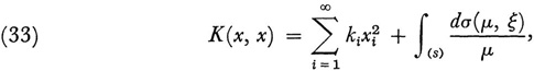
where the ki are the reciprocal eigenvalues of K. The integral, which we shall not describe further, is over a continuous range of eigenvalues or a continuous spectrum.
To eliminate the continuous spectrum, Hilbert introduces the concept of complete continuity. A function F(xi x2,…) of infinitely many variables is said to be completely continuous at a = (a1 a2…) if
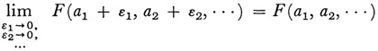
whenever ε1, ε2…, are allowed to run through any value system having the limit
This is a stronger requirement than continuity as previously introduced by Hilbert.
For a quadratic form K(x, x) to be completely continuous it is sufficient that 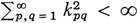 With the requirement of complete continuity, Hilbert is able to prove that if K is a completely continuous bounded form, then by an orthogonal transformation it can be brought into the form
where the kj are reciprocal eigenvalues and the (xi x2,,…) satisfy the condition that  is finite.
Now Hilbert applies his theory of quadratic forms in infinitely many variables to integral equations. The results in many instances are not new but are obtained by clearer and simpler methods. Hilbert starts this new work on integral equations by defining the important concept of a complete orthogonal system of functions (φ(s)}. This is a sequence of functions all defined and continuous on the interval [a, b] with the following properties:
(a) orthogonality:
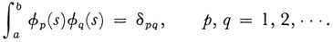
(b) completeness: for every pair of functions u and v defined on [a, b]
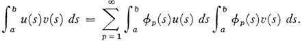
The value
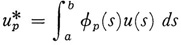
is called the Fourier coefficient of u(s) with respect to the system {φp}
Hilbert shows that a complete orthonormal system can be defined for any finite interval [a, b], for example, by the use of polynomials. Then a generalized Bessel’s inequality is proved, and finally the condition
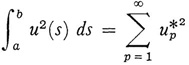
is shown to be equivalent to completeness.
Hilbert now turns to the integral equation

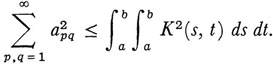
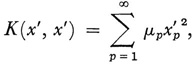
The kernel K(s, t), not necessarily symmetric, is developed in a double “Fourier” series by means of the coefficients
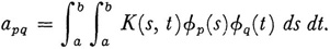
It follows that
Also, if
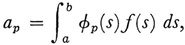
that is, if the ap are the “Fourier” coefficients oif(s), then 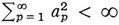
Hilbert next converts the above integral equation into a system of infinitely many linear equations in infinitely many unknowns. The idea is to look at solving the integral equation for φ(s) as a problem of finding the “Fourier” coefficients of φ(s). Denoting the as yet unknown coefficients by (x1, x2, he gets the following linear equations:
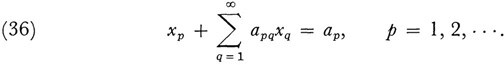
He proves that if this system has a unique solution, then the integral equation has a unique continuous solution, and when the linear homogeneous system associated with (36) has n linearly independent solutions, then the homogeneous integral equation associated with (35),

has n linearly independent solutions. In this case the original nonhomogeneous integral equation has a solution if and only if ψ(h)(s), h = 1, 2,…, n, which are the n linearly independent solutions of the transposed homogeneous equation
and which also exist when (37)has n solutions, satisfy the conditions

Thus the Fredholm alternative theorem is obtained: Either the equation
has a unique solution for all f or the associated homogeneous equation has n linearly independent solutions. In the latter case (39) has a solution if and only if the orthogonality conditions (38) are satisfied.
Hilbert turns next to the eigenvalue problem

where K is now symmetric. The symmetry of K implies that its “Fourier” coefficients determine a quadratic form K(x, x) which is completely continuous. He shows that there exists an orthogonal transformation T whose matrix is {lPq} such that
where the μp are the reciprocal eigenvalues of the quadratic form K(x, x). The eigenfunctions {φp(s)} for the kernel K(s, t) are now defined by
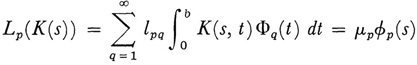
where the φp,(t) are a given complete orthonormal set. The φs(i) [as distinct from the φp(t)] are shown to form an orthonormal set and to satisfy
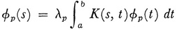
where λ„ = 1\μp. Thus Hilbert shows anew the existence of eigenfunctions for the homogeneous case of (40) and for every finite eigenvalue of the quadratic form K(x, x) associated with the kernel K(s, t) of (40).
Now Hilbert establishes again (Hilbert-Schmidt theorem) that if f(s) is any continuous function for which there is a g so that

then f is representable as a series in the eigenfunctions of K which is uniformly and absolutely convergent (cf. [31]). Hilbert uses this result to show that the homogeneous equation associated with (40) has no nontrivial solutions except at the eigenvalues λp. Then the Fredholm alternative theorem takes the form: For λ ≠ λp equation (40) has a unique solution. For λ ≠ λp, equation (40) has a solution if and only if the np conditions
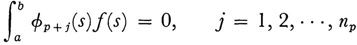
are satisfied where the φp + j(s) are the np eigenfunctions associated with λp. Finally, he proves anew the extension of the principal axis theorem:
where u(s) is an arbitrary (continuous) function and wherin all φp associated with any λp are included in the summation.
This later work (1906) of Hilbert dispensed with Fredholm’s infinite determinants. In it he showed directly the relation between integral equations and the theory of complete orthogonal systems and the expansion of functions in such systems.
Hilbert applied his results on integral equations to a variety of problems in geometry and physics. In particular, in the third of the six papers he solved Riemann’s problem of constructing a function holomorphic in a domain bounded by a smooth curve when the real or the imaginary part of the boundary value is given or both are related by a given linear equation.
One of the most noteworthy achievements in Hilbert’s work, which appears in the 1904 and 1905 papers, is the formulation of Sturm-Liouville boundary-value problems of differential equations as integral equations. Hilbert’s result states that the eigenvalues and eigenfunctions of the differential equation
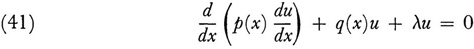
subject to the boundary conditions
u(a) = 0, e(b) = 0
(and even more general boundary conditions) are the eigenvalues and eigenfunctions of

where G(x, ξ) is the Green’s function for (41), that is, a particular solution of
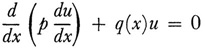
which satisfies certain differentiability conditions and whose first partial derivative ∂G/∂ has a jump singularity at x = ξ equal to –l/p(ξ). Similar results hold for partial differential equations. Thus integral equations are a way of solving ordinary and partial differential equations.
To recapitulate Hilbert‘s major results, first of all he established the
it had required great mathematical efforts (Chap. 28, sec. 8) to prove the existence of the lowest oscillating frequency for a membrane. With integral equations, constructive proof of the existence of the whole series of frequencies and of the actual eigenfunctions was obtained under very general conditions on the oscillating medium. These results were first derived, using Fredholm’s theory, by Emile Picard.15 Another noteworthy result due to Hilbert is that the development of a function in the eigenfunctions belonging to an integral equation of the second kind depends on the solvability of the corresponding integral equation of the first kind. In particular, Hilbert discovered that the success of Fredholm’s method rested on the notion of complete continuity, which he carried over to bilinear forms and studied intensively. Here he inaugurated the spectral theory of bilinear symmetric forms.
After Hilbert showed how to convert problems of differential equations to integral equations, this approach was used with increasing frequency to solve physical problems. Here the use of a Green’s function to convert has been a major tool. Also, Hilbert himself showed,16 in problems of gas dynamics, that one can go directly to integral equations. This direct recourse to integral equations is possible because the concept of summation proves as fundamental in some physical problems as the concept of rate of change which leads to differential equations is in other problems. Hilbert also emphasized that not ordinary or partial differential equations but integral equations are the necessary and natural starting point for the theory of expansion of functions in series, and that the expansions obtained through differential equations are just special cases of the general theorem in the theory of integral equations.
Hubert’s work on integral equations was simplified by Erhard Schmidt (1876-1959), professor at several German universities, who used methods originated by H. A. Schwarz in potential theory. Schmidt’s most significant contribution was his generalization in 1907 of the concept of eigenfunction to integral equations with non-symmetric kernels.17
Friedrich Riesz (1880-1956), a Hungarian professor of mathematics, in 1907 also took up Hubert’s work.18 Hilbert had treated integral equations of the form
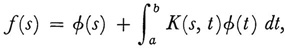
where f and K are continuous. Riesz sought to extend Hilbert’s ideas to more general functions f(s). Toward this end it was necessary to be sure that the “Fourier” coefficients of f could be determined with respect to a given orthonormal sequence of functions {φp}. He was also interested in discovering under what circumstances a given sequence of numbers {ap} could be the Fourier coefficients of some function f relative to a given orthonormal sequence {φp}.
Riesz introduced functions whose squares arc Lebesguc integrable and obtained the following theorem: Let be an orthonormal sequence of Lebcsgue square integrable functions all defined on the interval [a, b]. If {ap} is a sequence of real numbers, then the convergence of  is a necessary and sufficient condition for there to exist a function f such that
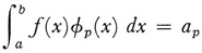
for each φp and ap. The function f proves to be Lebesgue square integrable. This theorem establishes a one-to-one correspondence between the set of Lebesgue square integrable functions and the set of square summable sequences through the mediation of any orthonormal sequence of Lebesgue square integrable functions.
With the introduction of Lebesgue integrable functions, Riesz was also able to show that the integral equation of the second kind
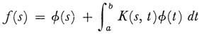
can be solved under the relaxed conditions that f(s) and K(s, t) are Lebesgue square integrable. Solutions are unique up to a function whose Lebesgue integral on [a, b] is 0.
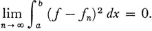
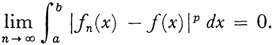
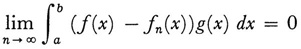
In the same year that Riesz published his first papers, Ernst Fischer (1875-1959), a professor at the University of Cologne, introduced the concept of convergence in the mean.19 A sequence of functions {fn} defined on an interval [a, b] is said to converge in the mean if
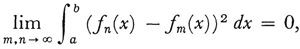
and {fn} is said to converge in the mean to f if
The integrals are Lebesgue integrals. The function f is uniquely determined to within a function defined over a set of measure 0, that is, a function g(x) ≠ 0, called a null function, which satisfies the condition 
The set of functions which are Lebesgue square integrable on an interval [a, b] was denoted later by L2(a, b) or simply by L2. Fischer’s main result is that L2[a, b) is complete in the mean; that is, if the functions fn belong to L2(a, b) and if {fn} converges in the mean, then there is a function f in L2(a, b) such that {fn} converges in the mean to f. This completeness property is the chief advantage of square summable functions. Fischer then deduced Riesz’s above theorem as a corollary, and this result is known as the Riesz-Fischer theorem. Fischer emphasized in a subsequent note20 that the use of Lebesgue square integrable functions was essential. No smaller set of functions would suffice.
The determination of a function f(x) that belongs to a given set of Fourier coefficients {an} with respect to a given sequence of orthonormal functions {g„}, or the determination of an f satisfying
which had arisen in Riesz’s 1907 works, is called the moment problem (Lebesgue integration is understood). In 191021 Riesz sought to generalize this problem. Because in this new work Riesz used the Holder inequalities
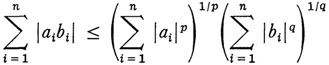
and
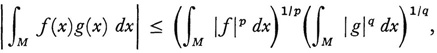
where l/p + 1/(q = 1, and other inequalities, he was obliged to introduce the set Lp of functions f measurable on a set M and for which |f|p is Lebesgue integrable on M. His first important theorem is that if a function h(x) is such that the product f(x)h(x) is integrable for every f in Lp, then h is in Lq and, conversely, the product of an LP function and an Lp function is always (Lebesgue) integrable. It is understood that p > 1 and 1/p + 1/q = 1.
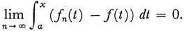
Riesz also introduced the concepts of strong and weak convergence. The sequence of functions (fn} is said to converge strongly to f (in the mean of order p) if
The sequence {fn} is said to converge weakly to f if
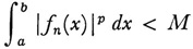
for M independent of n, and if for every x in [a, 6]
Strong convergence implies weak convergence. (The modern definition of weak convergence, if {fn} belongs to Lp and if f belongs to Lp and if
holds for every g in La, then {fn(x)} converges weakly to f, is equivalent to Riesz’s.)
In the same 1910 paper Riesz extended the theory of the integral equation
to the case where the given f and the unknown φ are functions in LP. The results on solution of the eigenvalue problem for this integral equation are analogous to Hubert’s results. What is more striking is that, to carry out his work, Riesz introduced the abstract concept of an operator, formulated for it the Hilbertian concept of complete continuity, and treated abstract operator theory. We shall say more about this abstract approach in the next chapter. Among other results, Riesz proved that the continuous spectrum of a real completely continuous operator in L2 is empty.
The importance Hilbert attached to integral equations made the subject a world-wide fad for a considerable length of time, and an enormous literature, most of it of ephemeral value, was produced. However, some extensions of the subject have proved valuable. We can merely name them.
The theory of integral equations presented above deals with linear integral equations; that is, the unknown function u(x) enters linearly. The theory has been extended to nonlinear integral equations, in which the unknown function enters to the second or higher degree or in some more complicated fashion.
Moreover, our brief sketch has said little about the conditions on the given functions f(x) and K(x, ξ) which lead to the many conclusions. If these functions are not continuous and the discontinuities are not limited, or if the interval [a, b] is replaced by an infinite interval, many of the results are altered or at least new proofs are needed. Thus even the Fourier transform
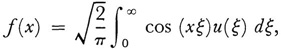
which can be regarded as an integral equation of the first kind and has as its solution the inverse transform
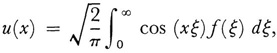
has just two eigenvalues ±1 and each has an infinite number of eigenfunctions. These cases are now studied under the heading of singular integral equations. Such equations cannot be solved by the methods applicable to the Volterra and Fredholm equations. Moreover, they exhibit a curious property, namely, there are continuous intervals of λ-values or band spectra for which there are solutions. The first significant paper on this subject is due to Hermann Weyl (1885-1955).22
The subject of existence theorems for integral equations has also been given a great deal of attention. This work has been devoted to linear and nonlinear integral equations. For example, existence theorems for
which includes as a special case the Volterra equation of the second kind
have been given by many mathematicians.
Historically, the next major development was an outgrowth of the work on integral equations. Hilbert regarded a function as given by its Fourier coefficients. These satisfy the condition that  is finite. He had also introduced sequences of real numbers {xn} such that
  is finite. Then Riesz and Fischer showed that there is a one-to-one correspondence between Lebesgue square summable functions and square summable sequences of their Fourier coefficients. The square summable sequences can be regarded as the coordinates of points in an infinite-dimensional space, which is a generalization of n-dimensional Euclidean space. Thus functions can be regarded as points of a space, now called Hilbert space, and the integral
 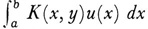 can be regarded as an operator transforming u(x) into itself or another function. These ideas suggested for the study of integral equations an abstract approach that fitted into an incipient abstract approach to the calculus of variations. This new approach is now known as functional analysis and we shall consider it next.
Bernkopf, M.: “The Development of Function Spaces with Particular Reference to their Origins in Integral Equation Theory,” Archive for History of Exact Sciences, 3, 1966, 1-96.
Bliss, G. A.: “The Scientific Work of E. H. Moore,” Amer. Math. Soc. Bull, 40, 1934, 501-14.
Bochcr, M.: An Introduction to the Study of Integral Equations, 2nd ed., Cambridge University Press, 1913.
Bourbaki, N.: Elements d’histoire des mathématiques, Hermann, 1960, pp. 230-45.
Davis, Harold T.: The Present State of Integral Equations, Indiana University Press, 1926.
Hahn, H.: “Bericht über die Theorie der linearen Integralgleichungen,” Jahres, der Deut. Math.-Verein., 20, 1911, 69-117.
Hellinger, E.: Hilberts Arbeiten über Integralgleichungen und unendliche Gleichungssysteme, in Hubert’s Gesam. Abh., 3, 94-145, Julius Springer, 1935.
________: “Begründung der Theorie quadratischer Formen von unendlichvielen Veränderlichen,” Jour, für Math., 136, 1909, 210-71.
Hellinger, E., and O. Tocplitz: “Integralgleichungen und Gleichungen mit unendlichvielen Unbekannten,” Encyk. der Math. Wiss., B. G. Teubner, 1923-27, Vol. 2, Part 3, 2nd half, 1335-1597.
Hilbert, D.: Grundzüge einer allgemeinen Theorie der linearen Integralgleichungen, 1912, Chelsea (reprint), 1953.
Reid, Constance: Hilbert, Springer-Verlag, 1970.
Volterra, Vito: Opere matematiche, 5 vols., Accademia Nazionale dei Lincei, 1954-62. Weyl, Hermann: Gesammelte Abhandlungen, 4 vols, Springer-Verlag, 1968.