CHAPTER 4
Sample Weights

4.1 Motivation

Chapter 3 presented several new methods for labeling financial observations. We introduced two novel concepts, the triple-barrier method and meta-labeling, and explained how they are useful in financial applications, including quantamental investment strategies. In this chapter you will learn how to use sample weights to address another problem ubiquitous in financial applications, namely that observations are not generated by independent and identically distributed (IID) processes. Most of the ML literature is based on the IID assumption, and one reason many ML applications fail in finance is because those assumptions are unrealistic in the case of financial time series.

4.2 Overlapping Outcomes

In Chapter 3 we assigned a label y_i to an observed feature X_i, where y_i was a function of price bars that occurred over an interval [t_{i, 0}, t_{i, 1}]. When t_{i, 1} > t_{j, 0} and i < j, then y_i and y_j will both depend on a common return , that is, the return over the interval [t_{j, 0}, min{t_{i, 1}, t_{j, 1}}]. The implication is that the series of labels, {y_i}_{i = 1, …, I}, are not IID whenever there is an overlap between any two consecutive outcomes, ∃i|t_{i, 1} > t_{i + 1, 0}..

Suppose that we circumvent this problem by restricting the bet horizon to t_{i, 1} ≤ t_{i + 1, 0}. In this case there is no overlap, because every feature outcome is determined before or at the onset of the next observed feature. That would lead to coarse models where the features’ sampling frequency would be limited by the horizon used to determine the outcome. On one hand, if we wished to investigate outcomes that lasted a month, features would have to be sampled with a frequency up to monthly. On the other hand, if we increased the sampling frequency to let's say daily, we would be forced to reduce the outcome's horizon to one day. Furthermore, if we wished to apply a path-dependent labeling technique, like the triple-barrier method, the sampling frequency would be subordinated to the first barrier's touch. No matter what you do, restricting the outcome's horizon to eliminate overlaps is a terrible solution. We must allow t_{i, 1} > t_{i + 1, 0}, which brings us back to the problem of overlapping outcomes described earlier.

This situation is characteristic of financial applications. Most non-financial ML researchers can assume that observations are drawn from IID processes. For example, you can obtain blood samples from a large number of patients, and measure their cholesterol. Of course, various underlying common factors will shift the mean and standard deviation of the cholesterol distribution, but the samples are still independent: There is one observation per subject. Suppose you take those blood samples, and someone in your laboratory spills blood from each tube into the following nine tubes to their right. That is, tube 10 contains blood for patient 10, but also blood from patients 1 through 9. Tube 11 contains blood from patient 11, but also blood from patients 2 through 10, and so on. Now you need to determine the features predictive of high cholesterol (diet, exercise, age, etc.), without knowing for sure the cholesterol level of each patient. That is the equivalent challenge that we face in financial ML, with the additional handicap that the spillage pattern is non-deterministic and unknown. Finance is not a plug-and-play subject as it relates to ML applications. Anyone who tells you otherwise will waste your time and money.

There are several ways to attack the problem of non-IID labels, and in this chapter we will address it by designing sampling and weighting schemes that correct for the undue influence of overlapping outcomes.

4.3 Number of Concurrent Labels

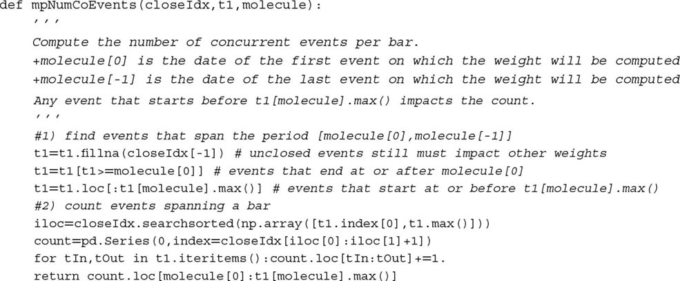
Two labels y_i and y_j are concurrent at t when both are a function of at least one common return, . The overlap does not need to be perfect, in the sense of both labels spanning the same time interval. In this section we are going to compute the number of labels that are a function of a given return, r_{t − 1, t}. First, for each time point t = 1, …, T, we form a binary array, {1_{t, i}}_{i = 1, …, I}, where 1_{t, i} ∈ {0, 1}. Variable 1_{t, i} = 1 if and only if [t_{i, 0}, t_{i, 1}] overlaps with [t − 1, t] and 1_{t, i} = 0 otherwise. Recall that the labels’ spans {[t_{i, 0}, t_{i, 1}]}_{i = 1, …, I} are defined by the t1 object introduced in Chapter 3. Second, we compute the number of labels concurrent at t, . Snippet 4.1 illustrates an implementation of this logic.

Snippet 4.1 Estimating the uniqueness of a label

4.4 Average Uniqueness of a Label

In this section we are going to estimate a label's uniqueness (non-overlap) as its average uniqueness over its lifespan. First, the uniqueness of a label i at time t is u_{t, i} = 1_{t, i}c^{− 1}_t. Second, the average uniqueness of label i is the average u_{t, i} over the label's lifespan, . This average uniqueness can also be interpreted as the reciprocal of the harmonic average of c_t over the event's lifespan. Figure 4.1 plots the histogram of uniqueness values derived from an object t1. Snippet 4.2 implements this calculation.

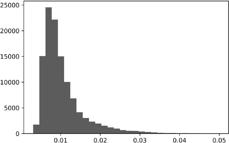
Figure 4.1 Histogram of uniqueness values

Snippet 4.2 Estimating the average uniqueness of a label

Note that we are making use again of the function mpPandasObj, which speeds up calculations via multiprocessing (see Chapter 20). Computing the average uniqueness associated with label i, , requires information that is not available until a future time, events['t1']. This is not a problem, because are used on the training set in combination with label information, and not on the testing set. These are not used for forecasting the label, hence there is no information leakage. This procedure allows us to assign a uniqueness score between 0 and 1 for each observed feature, in terms of non-overlapping outcomes.

4.5 Bagging Classifiers and Uniqueness

The probability of not selecting a particular item i after I draws with replacement on a set of I items is (1 − I^{− 1})^I. As the sample size grows, that probability converges to the asymptotic value . That means that the number of unique observations drawn is expected to be .

Suppose that the maximum number of non-overlapping outcomes is K ≤ I. Following the same argument, the probability of not selecting a particular item i after I draws with replacement on a set of I items is (1 − K^{− 1})^I. As the sample size grows, that probability can be approximated as . The number of times a particular item is sampled follows approximately a Poisson distribution with mean . The implication is that incorrectly assuming IID draws leads to oversampling.

When sampling with replacement (bootstrap) on observations with , it becomes increasingly likely that in-bag observations will be (1) redundant to each other, and (2) very similar to out-of-bag observations. Redundancy of draws makes the bootstrap inefficient (see Chapter 6). For example, in the case of a random forest, all trees in the forest will essentially be very similar copies of a single overfit decision tree. And because the random sampling makes out-of-bag examples very similar to the in-bag ones, out-of-bag accuracy will be grossly inflated. We will address this second issue in Chapter 7, when we study cross-validation under non-IID observations. For the moment, let us concentrate on the first issue, namely bagging under observations where .

A first solution is to drop overlapping outcomes before performing the bootstrap. Because overlaps are not perfect, dropping an observation just because there is a partial overlap will result in an extreme loss of information. I do not advise you to follow this solution.

A second and better solution is to utilize the average uniqueness, , to reduce the undue influence of outcomes that contain redundant information. Accordingly, we could sample only a fraction out['tW'].mean() of the observations, or a small multiple of that. In sklearn, the sklearn.ensemble.BaggingClassifier class accepts an argument max_samples, which can be set to max_samples=out['tW'].mean(). In this way, we enforce that the in-bag observations are not sampled at a frequency much higher than their uniqueness. Random forests do not offer that max_samples functionality, however, a solution is to bag a large number of decision trees. We will discuss this solution further in Chapter 6.

4.5.1 Sequential Bootstrap

A third and better solution is to perform a sequential bootstrap, where draws are made according to a changing probability that controls for redundancy. Rao et al. [1997] propose sequential resampling with replacement until K distinct original observations appear. Although interesting, their scheme does not fully apply to our financial problem. In the following sections we introduce an alternative method that addresses directly the problem of overlapping outcomes.

First, an observation X_i is drawn from a uniform distribution, i ∼ U[1, I], that is, the probability of drawing any particular value i is originally δ⁽¹⁾_i = I^{− 1}. For the second draw, we wish to reduce the probability of drawing an observation X_j with a highly overlapping outcome. Remember, a bootstrap allows sampling with repetition, so it is still possible to draw X_i again, but we wish to reduce its likelihood, since there is an overlap (in fact, a perfect overlap) between X_i and itself. Let us denote as φ the sequence of draws so far, which may include repetitions. Until now, we know that φ⁽¹⁾ = {i}. The uniqueness of j at time t is , as that is the uniqueness that results from adding alternative j’s to the existing sequence of draws φ⁽¹⁾. The average uniqueness of j is the average u⁽²⁾_{t, j} over j’s lifespan, . We can now make a second draw based on the updated probabilities {δ⁽²⁾_j}_{j = 1, …, I},

where {δ⁽²⁾_j}_{j = 1, .., I} are scaled to add up to 1, . We can now do a second draw, update φ⁽²⁾ and re-evaluate {δ⁽³⁾_j}_{j = 1, …, I}. The process is repeated until I draws have taken place. This sequential bootstrap scheme has the advantage that overlaps (even repetitions) are still possible, but decreasingly likely. The sequential bootstrap sample will be much closer to IID than samples drawn from the standard bootstrap method. This can be verified by measuring an increase in , relative to the standard bootstrap method.

4.5.2 Implementation of Sequential Bootstrap

Snippet 4.3 derives an indicator matrix from two arguments: the index of bars (barIx), and the pandas Series t1, which we used multiple times in Chapter 3. As a reminder, t1 is defined by an index containing the time at which the features are observed, and a values array containing the time at which the label is determined. The output of this function is a binary matrix indicating what (price) bars influence the label for each observation.

Snippet 4.3 Build an indicator matrix

Snippet 4.4 returns the average uniqueness of each observed feature. The input is the indicator matrix built by getIndMatrix.

Snippet 4.4 Compute average uniqueness

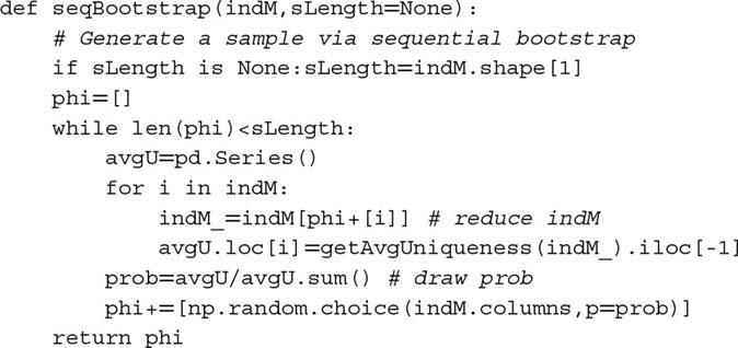
Snippet 4.5 gives us the index of the features sampled by sequential bootstrap. The inputs are the indicator matrix (indM) and an optional sample length (sLength), with a default value of as many draws as rows in indM.

Snippet 4.5 Return sample from sequential bootstrap

4.5.3 A Numerical Example

Consider a set of labels {y_i}_{i = 1, 2, 3}, where label y₁ is a function of return r_{0, 3}, label y₂ is a function of return r_{2, 4} and label y₃ is a function of return r_{4, 6}. The outcomes’ overlaps are characterized by this indicator matrix {1_{t, i}},

The procedure starts with φ⁽⁰⁾ = ∅, and a uniform distribution of probability, , ∀i = 1, 2, 3. Suppose that we randomly draw a number from {1, 2, 3}, and 2 is selected. Before we make a second draw on {1, 2, 3} (remember, a bootstrap samples with repetition), we need to adjust the probabilities. The set of observations drawn so far is φ⁽¹⁾ = {2}. The average uniqueness for the first feature is , and for the second feature is . The probabilities for the second draw are . Two points are worth mentioning: (1) The lowest probability goes to the feature that was picked in the first draw, as that would exhibit the highest overlap; and (2) among the two possible draws outside φ⁽¹⁾, the greater probability goes to δ⁽²⁾₃, as that is the label with no overlap to φ⁽¹⁾. Suppose that the second draw selects number 3. We leave as an exercise the update of the probabilities δ⁽³⁾ for the third and final draw. Snippet 4.6 runs a sequential bootstrap on the {1_{t, i}} indicator matrix in this example.

Snippet 4.6 Example of sequential bootstrap

4.5.4 Monte Carlo Experiments

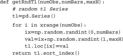
We can evaluate the efficiency of the sequential bootstrap algorithm through experimental methods. Snippet 4.7 lists the function that generates a random t1 series for a number of observations numObs (I). Each observation is made at a random number, drawn from a uniform distribution, with boundaries 0 and numBars, where numBars is the number of bars (T). The number of bars spanned by the observation is determined by drawing a random number from a uniform distribution with boundaries 0 and maxH.

Snippet 4.7 Generating a random t1 series

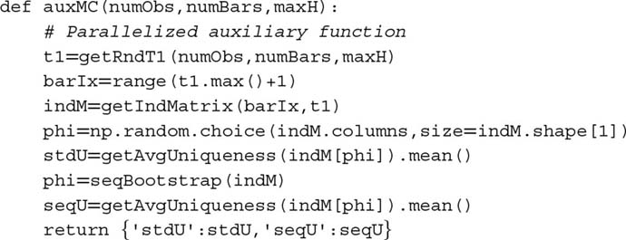
Snippet 4.8 takes that random t1 series, and derives the implied indicator matrix, indM. This matrix is then subjected to two procedures. In the first one, we derive the average uniqueness from a standard bootstrap (random sampling with replacement). In the second one, we derive the average uniqueness by applying our sequential bootstrap algorithm. Results are reported as a dictionary.

Snippet 4.8 Uniqueness from standard and sequential bootstraps

These operations have to be repeated over a large number of iterations. Snippet 4.9 implements this Monte Carlo using the multiprocessing techniques discussed in Chapter 20. For example, it will take about 6 hours for a 24-cores server to carry out a Monte Carlo of 1E6 iterations, where numObs=10, numBars=100, and maxH=5. Without parallelization, a similar Monte Carlo experiment would have taken about 6 days.

Snippet 4.9 Multi-threaded Monte Carlo

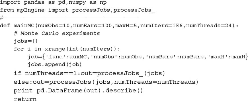
Figure 4.2 plots the histogram of the uniqueness from standard bootstrapped samples (left) and the sequentially bootstrapped samples (right). The median of the average uniqueness for the standard method is 0.6, and the median of the average uniqueness for the sequential method is 0.7. A one-sided t-test on the difference of means yields a vanishingly small probability. Statistically speaking, samples from the sequential bootstrap method have an expected uniqueness that exceeds that of the standard bootstrap method, at any reasonable confidence level.

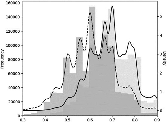
Figure 4.2 Monte Carlo experiment of standard vs. sequential bootstraps

4.6 Return Attribution

In the previous section we learned a method to bootstrap samples closer to IID. In this section we will introduce a method to weight those samples for the purpose of training an ML algorithm. Highly overlapping outcomes would have disproportionate weights if considered equal to non-overlapping outcomes. At the same time, labels associated with large absolute returns should be given more importance than labels with negligible absolute returns. In short, we need to weight observations by some function of both uniqueness and absolute return.

When labels are a function of the return sign ({ − 1, 1} for standard labeling or {0, 1} for meta-labeling), the sample weights can be defined in terms of the sum of the attributed returns over the event's lifespan, [t_{i, 0}, t_{i, 1}],

hence . We have scaled these weights to add up to I, since libraries (including sklearn) usually define algorithmic parameters assuming a default weight of 1.

The rationale for this method is that we wish to weight an observation as a function of the absolute log returns that can be attributed uniquely to it. However, this method will not work if there is a “neutral” (return below threshold) case. For that case, lower returns should be assigned higher weights, not the reciprocal. The “neutral” case is unnecessary, as it can be implied by a “−1” or “1” prediction with low confidence. This is one of several reasons I would generally advise you to drop “neutral” cases. Snippet 4.10 implements this method.

Snippet 4.10 Determination of sample weight by absolute return attribution

4.7 Time Decay

Markets are adaptive systems (Lo [2017]). As markets evolve, older examples are less relevant than the newer ones. Consequently, we would typically like sample weights to decay as new observations arrive. Let be the time-decay factors that will multiply the sample weights derived in the previous section. The final weight has no decay, , and all other weights will be adjusted relative to that. Let c ∈ ( − 1., .1] be a user-defined parameter that determines the decay function as follows: For c ∈ [0, 1], then d[1] = c, with linear decay; for c ∈ ( − 1, 0), then , with linear decay between and d[x] = 0 . For a linear piecewise function d = max{0, a + bx}, such requirements are met by the following boundary conditions:

1. .
2. Contingent on c:
   1. , ∀c ∈ [0, 1]
   2. , ∀c ∈ ( − 1, 0)

Snippet 4.11 implements this form of time-decay factors. Note that time is not meant to be chronological. In this implementation, decay takes place according to cumulative uniqueness, , because a chronological decay would reduce weights too fast in the presence of redundant observations.

Snippet 4.11 Implementation of time-decay factors

It is worth discussing a few interesting cases:

• c = 1 means that there is no time decay.
• 0 < c < 1 means that weights decay linearly over time, but every observation still receives a strictly positive weight, regardless of how old.
• c = 0 means that weights converge linearly to zero, as they become older.
• c < 0 means that the oldest portion cT of the observations receive zero weight (i.e., they are erased from memory).

Figure 4.3 shows the decayed weights, out['w']*df, after applying the decay factors for c ∈ {1, .75, .5, 0, −.25, −.5}. Although not necessarily practical, the procedure allows the possibility of generating weights that increase as they get older, by setting c > 1.

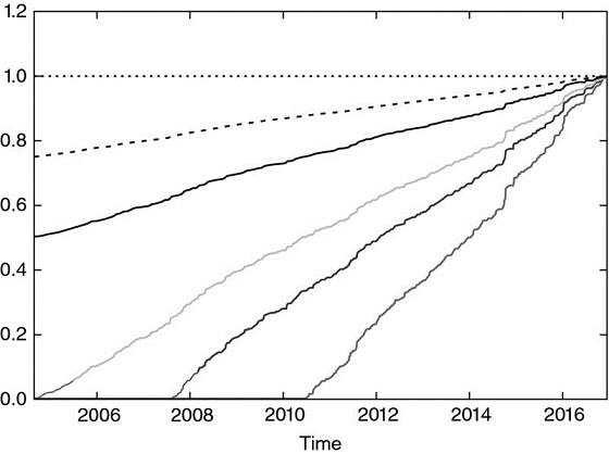
Figure 4.3 Piecewise-linear time-decay factors

4.8 Class Weights

In addition to sample weights, it is often useful to apply class weights. Class weights are weights that correct for underrepresented labels. This is particularly critical in classification problems where the most important classes have rare occurrences (King and Zeng [2001]). For example, suppose that you wish to predict liquidity crisis, like the flash crash of May 6, 2010. These events are rare relative to the millions of observations that take place in between them. Unless we assign higher weights to the samples associated with those rare labels, the ML algorithm will maximize the accuracy of the most common labels, and flash crashes will be deemed to be outliers rather than rare events.

ML libraries typically implement functionality to handle class weights. For example, sklearn penalizes errors in samples of class[j], j=1,…,J, with weighting class_weight[j] rather than 1. Accordingly, higher class weights on label j will force the algorithm to achieve higher accuracy on j. When class weights do not add up to J, the effect is equivalent to changing the regularization parameter of the classifier.

In financial applications, the standard labels of a classification algorithm are { − 1, 1}, where the zero (or neutral) case will be implied by a prediction with probability only slightly above 0.5 and below some neutral threshold. There is no reason for favoring accuracy of one class over the other, and as such a good default is to assign class_weight='balanced'. This choice re-weights observations so as to simulate that all classes appeared with equal frequency. In the context of bagging classifiers, you may want to consider the argument class_weight='balanced_subsample', which means that class_weight='balanced' will be applied to the in-bag bootstrapped samples, rather than to the entire dataset. For full details, it is helpful to read the source code implementing class_weight in sklearn. Please also be aware of this reported bug: https://github.com/scikit-learn/scikit-learn/issues/4324.

Exercises

1. In Chapter 3, we denoted as t1 a pandas series of timestamps where the first barrier was touched, and the index was the timestamp of the observation. This was the output of the getEvents function.

   1. Compute a t1 series on dollar bars derived from E-mini S&P 500 futures tick data.
   2. Apply the function mpNumCoEvents to compute the number of overlapping outcomes at each point in time.
   3. Plot the time series of the number of concurrent labels on the primary axis, and the time series of exponentially weighted moving standard deviation of returns on the secondary axis.
   4. Produce a scatterplot of the number of concurrent labels (x-axis) and the exponentially weighted moving standard deviation of returns (y-axis). Can you appreciate a relationship?

2. Using the function mpSampleTW, compute the average uniqueness of each label. What is the first-order serial correlation, AR(1), of this time series? Is it statistically significant? Why?

3. Fit a random forest to a financial dataset where .

   1. What is the mean out-of-bag accuracy?
   2. What is the mean accuracy of k-fold cross-validation (without shuffling) on the same dataset?
   3. Why is out-of-bag accuracy so much higher than cross-validation accuracy? Which one is more correct / less biased? What is the source of this bias?

4. Modify the code in Section 4.7 to apply an exponential time-decay factor.

5. Consider you have applied meta-labels to events determined by a trend-following model. Suppose that two thirds of the labels are 0 and one third of the labels are 1.

   1. What happens if you fit a classifier without balancing class weights?
   2. A label 1 means a true positive, and a label 0 means a false positive. By applying balanced class weights, we are forcing the classifier to pay more attention to the true positives, and less attention to the false positives. Why does that make sense?
   3. What is the distribution of the predicted labels, before and after applying balanced class weights?

6. Update the draw probabilities for the final draw in Section 4.5.3.

7. In Section 4.5.3, suppose that number 2 is picked again in the second draw. What would be the updated probabilities for the third draw?

References

1. Rao, C., P. Pathak and V. Koltchinskii (1997): “Bootstrap by sequential resampling.” Journal of Statistical Planning and Inference, Vol. 64, No. 2, pp. 257–281.
2. King, G. and L. Zeng (2001): “Logistic Regression in Rare Events Data.” Working paper, Harvard University. Available at https://gking.harvard.edu/files/0s.pdf.
3. Lo, A. (2017): Adaptive Markets, 1st ed. Princeton University Press.

Bibliography

Sample weighting is a common topic in the ML learning literature. However the practical problems discussed in this chapter are characteristic of investment applications, for which the academic literature is extremely scarce. Below are some publications that tangentially touch some of the issues discussed in this chapter.

1. Efron, B. (1979): “Bootstrap methods: Another look at the jackknife.” Annals of Statistics, Vol. 7, pp. 1–26.
2. Efron, B. (1983): “Estimating the error rote of a prediction rule: Improvement on cross-validation.” Journal of the American Statistical Association, Vol. 78, pp. 316–331.
3. Bickel, P. and D. Freedman (1981): “Some asymptotic theory for the bootstrap.” Annals of Statistics, Vol. 9, pp. 1196–1217.
4. Gine, E. and J. Zinn (1990): “Bootstrapping general empirical measures.” Annals of Probability, Vol. 18, pp. 851–869.
5. Hall, P. and E. Mammen (1994): “On general resampling algorithms and their performance in distribution estimation.” Annals of Statistics, Vol. 24, pp. 2011–2030.
6. Mitra, S. and P. Pathak (1984): “The nature of simple random sampling.” Annals of Statistics, Vol. 12, pp. 1536–1542.
7. Pathak, P. (1964): “Sufficiency in sampling theory.” Annals of Mathematical Statistics, Vol. 35, pp. 795–808.
8. Pathak, P. (1964): “On inverse sampling with unequal probabilities.” Biometrika, Vol. 51, pp. 185–193.
9. Praestgaard, J. and J. Wellner (1993): “Exchangeably weighted bootstraps of the general empirical process.” Annals of Probability, Vol. 21, pp. 2053–2086.
10. Rao, C., P. Pathak and V. Koltchinskii (1997): “Bootstrap by sequential resampling.” Journal of Statistical Planning and Inference, Vol. 64, No. 2, pp. 257–281.