CHAPTER 15
Understanding Strategy Risk
15.1 Motivation
As we saw in Chapters 3 and 13, investment strategies are often implemented in terms of positions held until one of two conditions are met: (1) a condition to exit the position with profits (profit-taking), or (2) a condition to exit the position with losses (stop-loss). Even when a strategy does not explicitly declare a stop-loss, there is always an implicit stop-loss limit, at which the investor can no longer finance her position (margin call) or bear the pain caused by an increasing unrealized loss. Because most strategies have (implicitly or explicitly) these two exit conditions, it makes sense to model the distribution of outcomes through a binomial process. This in turn will help us understand what combinations of betting frequency, odds, and payouts are uneconomic. The goal of this chapter is to help you evaluate when a strategy is vulnerable to small changes in any of these variables.
15.2 Symmetric Payouts
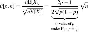
Consider a strategy that produces n IID bets per year, where the outcome Xi of a bet i ∈ [1, n] is a profit π > 0 with probability P[Xi = π] = p, and a loss − π with probability P[Xi = −π] = 1 − p. You can think of p as the precision of a binary classifier where a positive means betting on an opportunity, and a negative means passing on an opportunity: True positives are rewarded, false positives are punished, and negatives (whether true or false) have no payout. Since the betting outcomes {Xi}i = 1, …, n are independent, we will compute the expected moments per bet. The expected profit from one bet is E[Xi] = πp + ( − π)(1 − p) = π(2p − 1). The variance is V[Xi] = E[X2i] − E[Xi]2, where E[X2i] = π2p + ( − π)2(1 − p) = π2, thus V[Xi] = π2 − π2(2p − 1)2 = π2[1 − (2p − 1)2] = 4π2p(1 − p). For n IID bets per year, the annualized Sharpe ratio (θ) is

Note how π cancels out of the above equation, because the payouts are symmetric. Just as in the Gaussian case, θ[p, n] can be understood as a re-scaled t-value. This illustrates the point that, even for a small  , the Sharpe ratio can be made high for a sufficiently large n. This is the economic basis for high-frequency trading, where p can be barely above .5, and the key to a successful business is to increase n. The Sharpe ratio is a function of precision rather than accuracy, because passing on an opportunity (a negative) is not rewarded or punished directly (although too many negatives may lead to a small n, which will depress the Sharpe ratio toward zero).
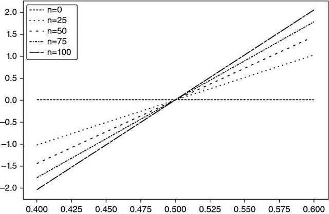
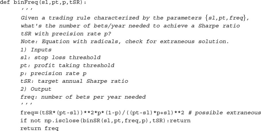
For example, for p = .55,  , and achieving an annualized Sharpe ratio of 2 requires 396 bets per year. Snippet 15.1 verifies this result experimentally. Figure 15.1 plots the Sharpe ratio as a function of precision, for various betting frequencies.

Figure 15.1 The relation between precision (x-axis) and sharpe ratio (y-axis) for various bet frequencies (n)
Snippet 15.1 Targeting a Sharpe ratio as a function of the number of bets

Solving for 0 ≤ p ≤ 1, we obtain  , with solution

This equation makes explicit the trade-off between precision (p) and frequency (n) for a given Sharpe ratio (θ). For example, a strategy that only produces weekly bets (n = 52) will need a fairly high precision of p = 0.6336 to deliver an annualized Sharpe of 2.
15.3 Asymmetric Payouts
Consider a strategy that produces n IID bets per year, where the outcome Xi of a bet i ∈ [1, n] is π+ with probability P[Xi = π+] = p, and an outcome π−, π− < π+ occurs with probability P[Xi = π−] = 1 − p. The expected profit from one bet is E[Xi] = pπ+ + (1 − p)π− = (π+ − π−)p + π−. The variance is V[Xi] = E[X2i] − E[Xi]2, where E[X2i] = pπ+2 + (1 − p)π2− = (π+2 − π2−)p + π−2, thus V[Xi] = (π+ − π−)2p(1 − p). For n IID bets per year, the annualized Sharpe ratio (θ) is

And for π− = −π+ we can see that this equation reduces to the symmetric case:  . For example, for n = 260, π− = −.01, π+ = .005, p = .7, we get θ = 1.173.
Finally, we can solve the previous equation for 0 ≤ p ≤ 1, to obtain

where:
- a = (n + θ2)(π+ − π−)2
- b = [2nπ− − θ2(π+ − π−)](π+ − π−)
- c = nπ2−
As a side note, Snippet 15.2 verifies these symbolic operations using SymPy Live: http://live.sympy.org/.
Snippet 15.2 Using the SymPy library for symbolic operations

The above equation answers the following question: Given a trading rule characterized by parameters {π−, π+, n}, what is the precision rate p required to achieve a Sharpe ratio of θ*? For example, for n = 260, π− = −.01, π+ = .005, in order to get θ = 2 we require a p = .72. Thanks to the large number of bets, a very small change in p (from p = .7 to p = .72) has propelled the Sharpe ratio from θ = 1.173 to θ = 2. On the other hand, this also tells us that the strategy is vulnerable to small changes in p. Snippet 15.3 implements the derivation of the implied precision. Figure 15.2 displays the implied precision as a function of n and π−, where π+ = 0.1 and θ* = 1.5. As π− becomes more negative for a given n, a higher p is required to achieve θ* for a given π+. As n becomes smaller for a given π−, a higher p is required to achieve θ* for a given π+.

Figure 15.2 Heat-map of the implied precision as a function of n and π−, with π+ = 0.1 and θ* = 1.5
Snippet 15.3 Computing the implied precision

Snippet 15.4 solves θ[p, n, π−, π+] for the implied betting frequency, n. Figure 15.3 plots the implied frequency as a function of p and π−, where π+ = 0.1 and θ* = 1.5. As π− becomes more negative for a given p, a higher n is required to achieve θ* for a given π+. As p becomes smaller for a given π−, a higher n is required to achieve θ* for a given π+.

Figure 15.3 Implied frequency as a function of p and, with = 0.1 and = 1.5
Snippet 15.4 Computing the implied betting frequency

15.4 The Probability of Strategy Failure
In the example above, parameters π− = −.01, π+ = .005 are set by the portfolio manager, and passed to the traders with the execution orders. Parameter n = 260 is also set by the portfolio manager, as she decides what constitutes an opportunity worth betting on. The two parameters that are not under the control of the portfolio manager are p (determined by the market) and θ* (the objective set by the investor). Because p is unknown, we can model it as a random variable, with expected value E[p]. Let us define  as the value of p below which the strategy will underperform a target Sharpe ratio θ*, that is,
  . We can use the equations above (or the binHR function) to conclude that for
  ,
,  . This highlights the risks involved in this strategy, because a relatively small drop in p (from p = .7 to p = .67) will wipe out all the profits. The strategy is intrinsically risky, even if the holdings are not. That is the critical difference we wish to establish with this chapter: Strategy risk should not be confused with portfolio risk.
Most firms and investors compute, monitor, and report portfolio risk without realizing that this tells us nothing about the risk of the strategy itself. Strategy risk is not the risk of the underlying portfolio, as computed by the chief risk officer. Strategy risk is the risk that the investment strategy will fail to succeed over time, a question of far greater relevance to the chief investment officer. The answer to the question “What is the probability that this strategy will fail?” is equivalent to computing  . The following algorithm will help us compute the strategy risk.
15.4.1 Algorithm
In this section we will describe a procedure to compute  . Given a time series of bet outcomes {πt}t = 1, …, T, first we estimate π− = E[{πt|πt ≤ 0}t = 1, …, T], and π+ = E[{πt|πt > 0}t = 1, …, T]. Alternatively, {π−, π+} could be derived from fitting a mixture of two Gaussians, using the EF3M algorithm (López de Prado and Foreman [2014]). Second, the annual frequency n is given by
  , where y is the number of years elapsed between t = 1 and t = T. Third, we bootstrap the distribution of p as follows:
- For iterations i = 1, …, I:
- Draw ⌊nk⌋ samples from {πt}t = 1, …, T with replacement, where k is the number of years used by investors to assess a strategy (e.g., 2 years). We denote the set of these drawn samples as {π(i)j}j = 1, …, ⌊nk⌋.
- Derive the observed precision from iteration i as
 .
.
- Fit the PDF of p, denoted f[p], by applying a Kernel Density Estimator (KDE) on {pi}i = 1, …, I.
For a sufficiently large k, we can approximate this third step as  , where
  . Fourth, given a threshold θ* (the Sharpe ratio that separates failure from success), derive
  (see Section 15.4). Fifth, the strategy risk is computed as
  .
.
15.4.2 Implementation
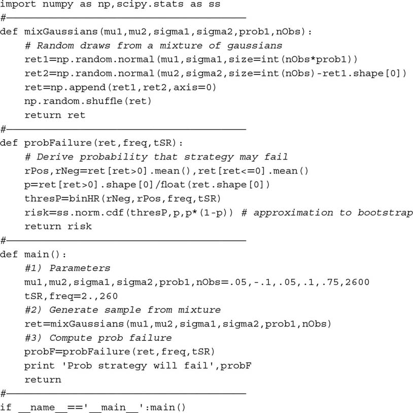
Snippet 15.5 lists one possible implementation of this algorithm. Typically we would disregard strategies where  as too risky, even if they invest in low volatility instruments. The reason is that even if they do not lose much money, the probability that they will fail to achieve their target is too high. In order to be deployed, the strategy developer must find a way to reduce
  .
.
Snippet 15.5 Calculating the strategy risk in practice

This approach shares some similarities with PSR (see Chapter 14, and Bailey and López de Prado [2012, 2014]). PSR derives the probability that the true Sharpe ratio exceeds a given threshold under non-Gaussian returns. Similarly, the method introduced in this chapter derives the strategy's probability of failure based on asymmetric binary outcomes. The key difference is that, while PSR does not distinguish between parameters under or outside the portfolio manager's control, the method discussed here allows the portfolio manager to study the viability of the strategy subject to the parameters under her control: {π−, π+, n}. This is useful when designing or assessing the viability of a trading strategy.
Exercises
-
A portfolio manager intends to launch a strategy that targets an annualized SR of 2. Bets have a precision rate of 60%, with weekly frequency. The exit conditions are 2% for profit-taking, and –2% for stop-loss.
- Is this strategy viable?
- Ceteris paribus, what is the required precision rate that would make the strategy profitable?
- For what betting frequency is the target achievable?
- For what profit-taking threshold is the target achievable?
- What would be an alternative stop-loss?
-
Following up on the strategy from exercise 1.
- What is the sensitivity of SR to a 1% change in each parameter?
- Given these sensitivities, and assuming that all parameters are equally hard to improve, which one offers the lowest hanging fruit?
- Does changing any of the parameters in exercise 1 impact the others? For example, does changing the betting frequency modify the precision rate, etc.?
-
Suppose a strategy that generates monthly bets over two years, with returns following a mixture of two Gaussian distributions. The first distribution has a mean of –0.1 and a standard deviation of 0.12. The second distribution has a mean of 0.06 and a standard deviation of 0.03. The probability that a draw comes from the first distribution is 0.15.
- Following López de Prado and Peijan [2004] and López de Prado and Foreman [2014], derive the first four moments for the mixture's returns.
- What is the annualized SR?
- Using those moments, compute PSR[1] (see Chapter 14). At a 95% confidence level, would you discard this strategy?
-
Using Snippet 15.5, compute
 for the strategy described in exercise 3. At a significance level of 0.05, would you discard this strategy? Is this result consistent with PSR[θ*]?
 -
In general, what result do you expect to be more accurate, PSR[θ*] or
 ? How are these two methods complementary?
 -
Re-examine the results from Chapter 13, in light of what you have learned in this chapter.
- Does the asymmetry between profit taking and stop-loss thresholds in OTRs make sense?
- What is the range of p implied by Figure 13.1, for a daily betting frequency?
- What is the range of p implied by Figure 13.5, for a weekly betting frequency?
References
- Bailey, D. and M. López de Prado (2014): “The deflated Sharpe ratio: Correcting for selection bias, backtest overfitting and non-normality.” Journal of Portfolio Management, Vol. 40, No. 5. Available at https://ssrn.com/abstract=2460551.
- Bailey, D. and M. López de Prado (2012): “The Sharpe ratio efficient frontier.” Journal of Risk, Vol. 15, No. 2, pp. 3–44. Available at https://ssrn.com/abstract=1821643.
- López de Prado, M. and M. Foreman (2014): “A mixture of Gaussians approach to mathematical portfolio oversight: The EF3M algorithm.” Quantitative Finance, Vol. 14, No. 5, pp. 913–930. Available at https://ssrn.com/abstract=1931734.
- López de Prado, M. and A. Peijan (2004): “Measuring loss potential of hedge fund strategies.” Journal of Alternative Investments, Vol. 7, No. 1 (Summer), pp. 7–31. Available at http://ssrn.com/abstract=641702.