CHAPTER 16
Machine Learning Asset Allocation

16.1 Motivation

This chapter introduces the Hierarchical Risk Parity (HRP) approach.1 HRP portfolios address three major concerns of quadratic optimizers in general and Markowitz's Critical Line Algorithm (CLA) in particular: instability, concentration, and underperformance. HRP applies modern mathematics (graph theory and machine learning techniques) to build a diversified portfolio based on the information contained in the covariance matrix. However, unlike quadratic optimizers, HRP does not require the invertibility of the covariance matrix. In fact, HRP can compute a portfolio on an ill-degenerated or even a singular covariance matrix, an impossible feat for quadratic optimizers. Monte Carlo experiments show that HRP delivers lower out-of-sample variance than CLA, even though minimum-variance is CLA's optimization objective. HRP produces less risky portfolios out-of-sample compared to traditional risk parity methods. Historical analyses have also shown that HRP would have performed better than standard approaches (Kolanovic et al. [2017], Raffinot [2017]). A practical application of HRP is to determine allocations across multiple machine learning (ML) strategies.

16.2 The Problem with Convex Portfolio Optimization

Portfolio construction is perhaps the most recurrent financial problem. On a daily basis, investment managers must build portfolios that incorporate their views and forecasts on risks and returns. This is the primordial question that 24-year-old Harry Markowitz attempted to answer more than six decades ago. His monumental insight was to recognize that various levels of risk are associated with different optimal portfolios in terms of risk-adjusted returns, hence the notion of “efficient frontier” (Markowitz [1952]). One implication is that it is rarely optimal to allocate all assets to the investments with highest expected returns. Instead, we should take into account the correlations across alternative investments in order to build a diversified portfolio.

Before earning his PhD in 1954, Markowitz left academia to work for the RAND Corporation, where he developed the Critical Line Algorithm. CLA is a quadratic optimization procedure specifically designed for inequality-constrained portfolio optimization problems. This algorithm is notable in that it guarantees that the exact solution is found after a known number of iterations, and that it ingeniously circumvents the Karush-Kuhn-Tucker conditions (Kuhn and Tucker [1951]). A description and open-source implementation of this algorithm can be found in Bailey and López de Prado [2013]. Surprisingly, most financial practitioners still seem unaware of CLA, as they often rely on generic-purpose quadratic programming methods that do not guarantee the correct solution or a stopping time.

Despite of the brilliance of Markowitz's theory, a number of practical problems make CLA solutions somewhat unreliable. A major caveat is that small deviations in the forecasted returns will cause CLA to produce very different portfolios (Michaud [1998]). Given that returns can rarely be forecasted with sufficient accuracy, many authors have opted for dropping them altogether and focusing on the covariance matrix. This has led to risk-based asset allocation approaches, of which “risk parity” is a prominent example (Jurczenko [2015]). Dropping the forecasts on returns improves but does not prevent the instability issues. The reason is that quadratic programming methods require the inversion of a positive-definite covariance matrix (all eigenvalues must be positive). This inversion is prone to large errors when the covariance matrix is numerically ill-conditioned, that is, when it has a high condition number (Bailey and López de Prado [2012]).

16.3 Markowitz's Curse

The condition number of a covariance, correlation (or normal, thus diagonalizable) matrix is the absolute value of the ratio between its maximal and minimal (by moduli) eigenvalues. Figure 16.1 plots the sorted eigenvalues of several correlation matrices, where the condition number is the ratio between the first and last values of each line. This number is lowest for a diagonal correlation matrix, which is its own inverse. As we add correlated (multicollinear) investments, the condition number grows. At some point, the condition number is so high that numerical errors make the inverse matrix too unstable: A small change on any entry will lead to a very different inverse. This is Markowitz's curse: The more correlated the investments, the greater the need for diversification, and yet the more likely we will receive unstable solutions. The benefits of diversification often are more than offset by estimation errors.

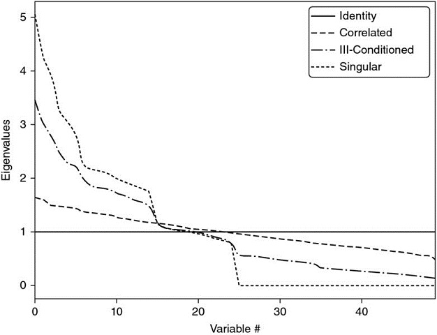
Figure 16.1 Visualization of Markowitz's curse
A diagonal correlation matrix has the lowest condition number. As we add correlated investments, the maximum eigenvalue is greater and the minimum eigenvalue is lower. The condition number rises quickly, leading to unstable inverse correlation matrices. At some point, the benefits of diversification are more than offset by estimation errors.

Increasing the size of the covariance matrix will only make matters worse, as each covariance coefficient is estimated with fewer degrees of freedom. In general, we need at least independent and identically distributed (IID) observations in order to estimate a covariance matrix of size N that is not singular. For example, estimating an invertible covariance matrix of size 50 requires, at the very least, 5 years of daily IID data. As most investors know, correlation structures do not remain invariant over such long periods by any reasonable confidence level. The severity of these challenges is epitomized by the fact that even naïve (equally-weighted) portfolios have been shown to beat mean-variance and risk-based optimization out-of-sample (De Miguel et al. [2009]).

16.4 From Geometric to Hierarchical Relationships

These instability concerns have received substantial attention in recent years, as Kolm et al. [2014] have carefully documented. Most alternatives attempt to achieve robustness by incorporating additional constraints (Clarke et al. [2002]), introducing Bayesian priors (Black and Litterman [1992]), or improving the numerical stability of the covariance matrix's inverse (Ledoit and Wolf [2003]).

All the methods discussed so far, although published in recent years, are derived from (very) classical areas of mathematics: geometry, linear algebra, and calculus. A correlation matrix is a linear algebra object that measures the cosines of the angles between any two vectors in the vector space formed by the returns series (see Calkin and López de Prado [2014a, 2015b]). One reason for the instability of quadratic optimizers is that the vector space is modelled as a complete (fully connected) graph, where every node is a potential candidate to substitute another. In algorithmic terms, inverting the matrix means evaluating the partial correlations across the complete graph. Figure 16.2(a) visualizes the relationships implied by a covariance matrix of 50 × 50, that is 50 nodes and 1225 edges. This complex structure magnifies small estimation errors, leading to incorrect solutions. Intuitively, it would be desirable to drop unnecessary edges.

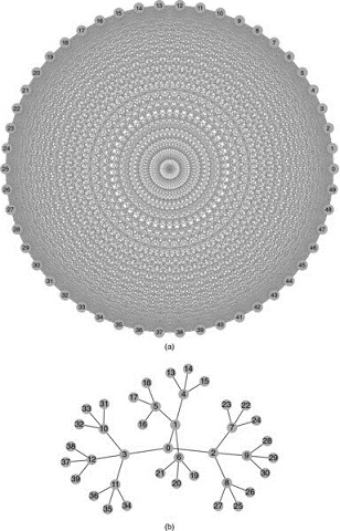
Figure 16.2 The complete-graph (top) and the tree-graph (bottom) structures
Correlation matrices can be represented as complete graphs, which lack the notion of hierarchy: Each investment is substitutable with another. In contrast, tree structures incorporate hierarchical relationships.

Let us consider for a moment the practical implications of such a topological structure. Suppose that an investor wishes to build a diversified portfolio of securities, including hundreds of stocks, bonds, hedge funds, real estate, private placements, etc. Some investments seem closer substitutes of one another, and other investments seem complementary to one another. For example, stocks could be grouped in terms of liquidity, size, industry, and region, where stocks within a given group compete for allocations. In deciding the allocation to a large publicly traded U.S. financial stock like J. P. Morgan, we will consider adding or reducing the allocation to another large publicly traded U.S. bank like Goldman Sachs, rather than a small community bank in Switzerland, or a real estate holding in the Caribbean. Yet, to a correlation matrix, all investments are potential substitutes to one another. In other words, correlation matrices lack the notion of hierarchy. This lack of hierarchical structure allows weights to vary freely in unintended ways, which is a root cause of CLA's instability. Figure 16.2(b) visualizes a hierarchical structure known as a tree. A tree structure introduces two desirable features: (1) It has only N − 1 edges to connect N nodes, so the weights only rebalance among peers at various hierarchical levels; and (2) the weights are distributed top-down, consistent with how many asset managers build their portfolios (e.g., from asset class to sectors to individual securities). For these reasons, hierarchical structures are better designed to give not only stable but also intuitive results.

In this chapter we will study a new portfolio construction method that addresses CLA's pitfalls using modern mathematics: graph theory and machine learning. This Hierarchical Risk Parity method uses the information contained in the covariance matrix without requiring its inversion or positive-definitiveness. HRP can even compute a portfolio based on a singular covariance matrix. The algorithm operates in three stages: tree clustering, quasi-diagonalization, and recursive bisection.

16.4.1 Tree Clustering

Consider a TxN matrix of observations X, such as returns series of N variables over T periods. We would like to combine these N column-vectors into a hierarchical structure of clusters, so that allocations can flow downstream through a tree graph.

First, we compute an NxN correlation matrix with entries ρ = {ρ_{i, j}}_{i, j = 1, …, N}, where ρ_{i, j} = ρ[X_i, X_j]. We define the distance measure , , where B is the Cartesian product of items in {1, …, i, …, N}. This allows us to compute an NxN distance matrix D = {d_{i, j}}_{i, j = 1, …, N}. Matrix D is a proper metric space (see Appendix 16.A.1 for a proof), in the sense that d[x, y] ≥ 0 (non-negativity), d[x, y] = 0⇔X = Y (coincidence), d[x, y] = d[Y, X] (symmetry), and d[X, Z] ≤ d[x, y] + d[Y, Z] (sub-additivity). See Example 16.1.

Example 16.1 Encoding a correlation matrix ρ as a distance matrix D

Second, we compute the Euclidean distance between any two column-vectors of D, , . Note the difference between distance metrics d_{i, j} and . Whereas d_{i, j} is defined on column-vectors of X, is defined on column-vectors of D (a distance of distances). Therefore, is a distance defined over the entire metric space D, as each is a function of the entire correlation matrix (rather than a particular cross-correlation pair). See Example 16.2.

Example 16.2 Euclidean distance of correlation distances

Third, we cluster together the pair of columns (i*, j*) such that , and denote this cluster as u[1]. See Example 16.3.

Example 16.3 Clustering items

Fourth, we need to define the distance between a newly formed cluster u[1] and the single (unclustered) items, so that may be updated. In hierarchical clustering analysis, this is known as the “linkage criterion.” For example, we can define the distance between an item i of and the new cluster u[1] as (the nearest point algorithm). See Example 16.4.

Example 16.4 Updating matrix with the new cluster u

Fifth, matrix is updated by appending and dropping the clustered columns and rows j ∈ u[1]. See Example 16.5.

Example 16.5 Updating matrix with the new cluster u

Sixth, applied recursively, steps 3, 4, and 5 allow us to append N − 1 such clusters to matrix D, at which point the final cluster contains all of the original items, and the clustering algorithm stops. See Example 16.6.

Example 16.6 Recursion in search of remaining clusters

Figure 16.3 displays the clusters formed at each iteration for this example, as well as the distances that triggered every cluster (third step). This procedure can be applied to a wide array of distance metrics d_{i, j}, and , beyond those illustrated in this chapter. See Rokach and Maimon [2005] for alternative metrics, the discussion on Fiedler's vector and Stewart's spectral clustering method in Brualdi [2010], as well as algorithms in the scipy library.² Snippet 16.1 provides an example of tree clustering using scipy functionality.

Figure 16.3 Sequence of cluster formation
A tree structure derived from our numerical example, here plotted as a dendogram. The y-axis measures the distance between the two merging leaves.

Snippet 16.1 Tree clustering using scipy functionality

This stage allows us to define a linkage matrix as an (N − 1)x4 matrix with structure Y = {(y_{m, 1}, y_{m, 2}, y_{m, 3}, y_{m, 4})}_{m = 1, …, N − 1} (i.e., with one 4-tuple per cluster). Items (y_{m, 1}, y_{m, 2}) report the constituents. Item y_{m, 3} reports the distance between y_{m, 1} and y_{m, 2}, that is . Item y_{m, 4} ≤ N reports the number of original items included in cluster m.

16.4.2 Quasi-Diagonalization

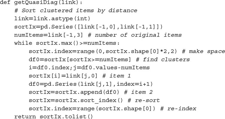
This stage reorganizes the rows and columns of the covariance matrix, so that the largest values lie along the diagonal. This quasi-diagonalization of the covariance matrix (without requiring a change of basis) renders a useful property: Similar investments are placed together, and dissimilar investments are placed far apart (see Figures 16.5 and 16.6 for an example). The algorithm works as follows: We know that each row of the linkage matrix merges two branches into one. We replace clusters in (y_{N − 1, 1}, y_{N − 1, 2}) with their constituents recursively, until no clusters remain. These replacements preserve the order of the clustering. The output is a sorted list of original (unclustered) items. This logic is implemented in Snippet 16.2.

Snippet 16.2 Quasi-diagonalization

16.4.3 Recursive Bisection

Stage 2 has delivered a quasi-diagonal matrix. The inverse-variance allocation is optimal for a diagonal covariance matrix (see Appendix 16.A.2 for a proof). We can take advantage of these facts in two different ways: (1) bottom-up, to define the variance of a contiguous subset as the variance of an inverse-variance allocation; or (2) top-down, to split allocations between adjacent subsets in inverse proportion to their aggregated variances. The following algorithm formalizes this idea:

1. The algorithm is initialized by:
   1. setting the list of items: L = {L₀}, with L₀ = {n}_{n = 1, …, N}
   2. assigning a unit weight to all items: w_n = 1, ∀n = 1, …, N
2. If |L_i| = 1,  ∀L_i ∈ L, then stop.
3. For each L_i ∈ L such that |L_i| > 1:
   1. bisect L_i into two subsets, L⁽¹⁾_i∪L_i⁽²⁾ = L_i, where , and the order is preserved
   2. define the variance of L^(j)_i, j = 1, 2, as the quadratic form , where V^(j)_i is the covariance matrix between the constituents of the L^(j)_i bisection, and , where diag[.] and tr[.] are the diagonal and trace operators
   3. compute the split factor: , so that 0 ≤ α_i ≤ 1
   4. re-scale allocations w_n by a factor of α_i, ∀n ∈ L⁽¹⁾_i
   5. re-scale allocations w_n by a factor of (1 − α_i), ∀n ∈ L⁽²⁾_i
4. Loop to step 2

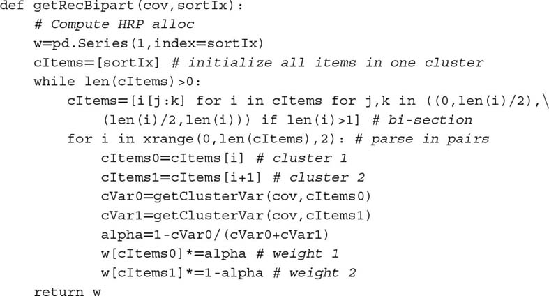
Step 3b takes advantage of the quasi-diagonalization bottom-up, because it defines the variance of the partition L^(j)_i using inverse-variance weightings . Step 3c takes advantage of the quasi-diagonalization top-down, because it splits the weight in inverse proportion to the cluster's variance. This algorithm guarantees that 0 ≤ w_i ≤ 1, ∀i = 1, …, N, and , because at each iteration we are splitting the weights received from higher hierarchical levels. Constraints can be easily introduced in this stage, by replacing the equations in steps 3c, 3d, and 3e according to the user's preferences. Stage 3 is implemented in Snippet 16.3.

Snippet 16.3 Recursive bisection

This concludes a first description of the HRP algorithm, which solves the allocation problem in best-case deterministic logarithmic time, , and worst-case deterministic linear time, . Next, we will put to practice what we have learned, and evaluate the method's accuracy out-of-sample.

16.5 A Numerical Example

We begin by simulating a matrix of observations X, of order (10000x10). The correlation matrix is visualized in Figure 16.4 as a heatmap. Figure 16.5 displays the dendogram of the resulting clusters (stage 1). Figure 16.6 shows the same correlation matrix, reorganized in blocks according to the identified clusters (stage 2). Appendix 16.A.3 provides the code used to generate this numerical example.

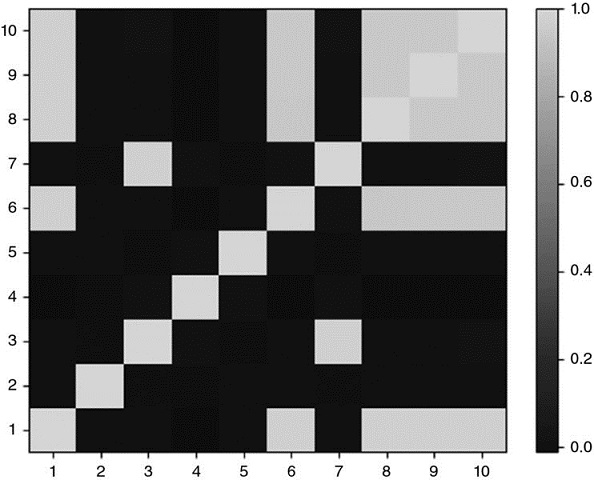
Figure 16.4 Heat-map of original covariance matrix
This correlation matrix has been computed using function generateData from snippet 16.4 (see Section 16.A.3). The last five columns are partially correlated to some of the first five series.

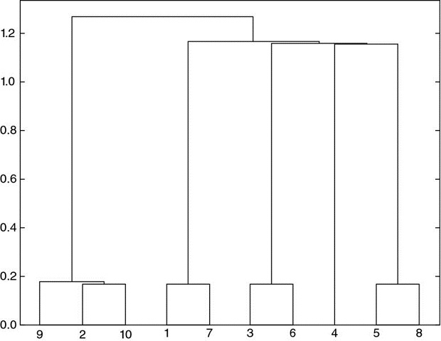
Figure 16.5 Dendogram of cluster formation
The clustering procedure has correctly identified that series 9 and 10 were perturbations of series 2, hence (9, 2, 10) are clustered together. Similarly, 7 is a perturbation of 1, 6 is a perturbation of 3, and 8 is a perturbation of 5. The only original item that was not perturbated is 4, and that is the one item for which the clustering algorithm found no similarity.

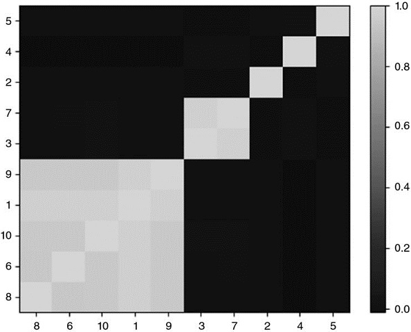
Figure 16.6 Clustered covariance matrix
Stage 2 quasi-diagonalizes the correlation matrix, in the sense that the largest values lie along the diagonal. However, unlike PCA or similar procedures, HRP does not require a change of basis. HRP solves the allocation problem robustly, while working with the original investments.

On this random data, we compute HRP's allocations (stage 3), and compare them to the allocations from two competing methodologies: (1) Quadratic optimization, as represented by CLA's minimum-variance portfolio (the only portfolio of the efficient frontier that does not depend on returns’ means); and (2) traditional risk parity, exemplified by the Inverse-Variance Portfolio (IVP). See Bailey and López de Prado [2013] for a comprehensive implementation of CLA, and Appendix 16.A.2 for a derivation of IVP. We apply the standard constraints that 0 ≤ w_i ≤ 1 (non-negativity), ∀i = 1, …, N, and (full investment). Incidentally, the condition number for the covariance matrix in this example is only 150.9324, not particularly high and therefore not unfavorable to CLA.

From the allocations in Table 16.1, we can appreciate a few stylized features: First, CLA concentrates 92.66% of the allocation on the top-5 holdings, while HRP concentrates only 62.57%. Second, CLA assigns zero weight to 3 investments (without the 0 ≤ w_i constraint, the allocation would have been negative). Third, HRP seems to find a compromise between CLA's concentrated solution and traditional risk parity's IVP allocation. The reader can use the code in Appendix 16.A.3 to verify that these findings generally hold for alternative random covariance matrices.

Table 16.1 A Comparison of Three Allocations

Weight #	CLA	HRP	IVP
1	14.44%	7.00%	10.36%
2	19.93%	7.59%	10.28%
3	19.73%	10.84%	10.36%
4	19.87%	19.03%	10.25%
5	18.68%	9.72%	10.31%
6	0.00%	10.19%	9.74%
7	5.86%	6.62%	9.80%
8	1.49%	9.10%	9.65%
9	0.00%	7.12%	9.64%
10	0.00%	12.79%	9.61%

A characteristic outcome of the three methods studied: CLA concentrates weights on a few investments, hence becoming exposed to idiosyncratic shocks. IVP evenly spreads weights through all investments, ignoring the correlation structure. This makes it vulnerable to systemic shocks. HRP finds a compromise between diversifying across all investments and diversifying across cluster, which makes it more resilient against both types of shocks.

What drives CLA's extreme concentration is its goal of minimizing the portfolio's risk. And yet both portfolios have a very similar standard deviation (σ_HRP = 0.4640, σ_CLA = 0.4486). So CLA has discarded half of the investment universe in favor of a minor risk reduction. The reality of course is that CLA's portfolio is deceitfully diversified, because any distress situation affecting the top-5 allocations will have a much greater negative impact on CLA's than on HRP's portfolio.

16.6 Out-of-Sample Monte Carlo Simulations

In our numerical example, CLA's portfolio has lower risk than HRP's in-sample. However, the portfolio with minimum variance in-sample is not necessarily the one with minimum variance out-of-sample. It would be all too easy for us to pick a particular historical dataset where HRP outperforms CLA and IVP (see Bailey and López de Prado [2014], and recall our discussion of selection bias in Chapter 11). Instead, in this section we follow the backtesting paradigm explained in Chapter 13, and evaluate via Monte Carlo the performance out-of-sample of HRP against CLA's minimum-variance and traditional risk parity's IVP allocations. This will also help us understand what features make a method preferable to the rest, regardless of anecdotal counter-examples.

First, we generate 10 series of random Gaussian returns (520 observations, equivalent to 2 years of daily history), with 0 mean and an arbitrary standard deviation of 10%. Real prices exhibit frequent jumps (Merton [1976]) and returns are not cross-sectionally independent, so we must add random shocks and a random correlation structure to our generated data. Second, we compute HRP, CLA, and IVP portfolios by looking back at 260 observations (a year of daily history). These portfolios are re-estimated and rebalanced every 22 observations (equivalent to a monthly frequency). Third, we compute the out-of-sample returns associated with those three portfolios. This procedure is repeated 10,000 times.

All mean portfolio returns out-of-sample are essentially 0, as expected. The critical difference comes from the variance of the out-of-sample portfolio returns: σ²_CLA = 0.1157, σ²_IVP = 0.0928, and σ²_HRP = 0.0671. Although CLA's goal is to deliver the lowest variance (that is the objective of its optimization program), its performance happens to exhibit the highest variance out-of-sample, and 72.47% greater variance than HRP's. This experimental finding is consistent with the historical evidence in De Miguel et al. [2009]. In other words, HRP would improve the out-of-sample Sharpe ratio of a CLA strategy by about 31.3%, a rather significant boost. Assuming that the covariance matrix is diagonal brings some stability to the IVP; however, its variance is still 38.24% greater than HRP's. This variance reduction out-of-sample is critically important to risk parity investors, given their use of substantial leverage. See Bailey et al. [2014] for a broader discussion of in-sample vs. out-of-sample performance.

The mathematical proof for HRP's outperformance over Markowitz's CLA and traditional risk parity's IVP is somewhat involved and beyond the scope of this chapter. In intuitive terms, we can understand the above empirical results as follows: Shocks affecting a specific investment penalize CLA's concentration. Shocks involving several correlated investments penalize IVP's ignorance of the correlation structure. HRP provides better protection against both common and idiosyncratic shocks by finding a compromise between diversification across all investments and diversification across clusters of investments at multiple hierarchical levels. Figure 16.7 plots the time series of allocations for the first of the 10,000 runs.

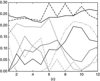
Figure 16.7 (a) Time series of allocations for IVP.
Between the first and second rebalance, one investment receives an idiosyncratic shock, which increases its variance. IVP's response is to reduce the allocation to that investment, and spread that former exposure across all other investments. Between the fifth and sixth rebalance, two investments are affected by a common shock. IVP's response is the same. As a result, allocations among the seven unaffected investments grow over time, regardless of their correlation.
(b) Time series of allocations for HRP
HRP's response to the idiosyncratic shock is to reduce the allocation to the affected investment, and use that reduced amount to increase the allocation to a correlated investment that was unaffected. As a response to the common shock, HRP reduces allocation to the affected investments and increases allocation to uncorrelated ones (with lower variance).
(c) Time series of allocations for CLA
CLA allocations respond erratically to idiosyncratic and common shocks. If we had taken into account rebalancing costs, CLA's performance would have been very negative.

Appendix 16.A.4 provides the Python code that implements the above study. The reader can experiment with different parameter configurations and reach similar conclusions. In particular, HRP's out-of-sample outperformance becomes even more substantial for larger investment universes, or when more shocks are added, or a stronger correlation structure is considered, or rebalancing costs are taken into account. Each of these CLA rebalances incurs transaction costs that can accumulate into prohibitive losses over time.

16.7 Further Research

The methodology introduced in this chapter is flexible, scalable and admits multiple variations of the same ideas. Using the code provided, readers can research and evaluate what HRP configurations work best for their particular problem. For example, at stage 1 they can apply alternative definitions of d_{i, j}, and , or different clustering algorithms, like biclustering; at stage 3, they can use different functions for and α, or alternative allocation constraints. Instead of carrying out a recursive bisection, stage 3 could also split allocations top-down using the clusters from stage 1.

It is relatively straightforward to incorporate forecasted returns, Ledoit-Wolf shrinkage, and Black-Litterman–style views to this hierarchical approach. In fact, the inquisitive reader may have realized that, at its core, HRP is essentially a robust procedure to avoid matrix inversions, and the same ideas underlying HRP can be used to replace many econometric regression methods, notorious for their unstable outputs (like VAR or VECM). Figure 16.8 displays (a) a large correlation matrix of fixed income securities before and (b) after clustering, with over 2.1 million entries. Traditional optimization or econometric methods fail to recognize the hierarchical structure of financial Big Data, where the numerical instabilities defeat the benefits of the analysis, resulting in unreliable and detrimental outcomes.

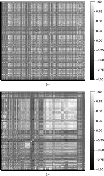
Figure 16.8 Correlation matrix before and after clustering
The methodology described in this chapter can be applied to problems beyond optimization. For example, a PCA analysis of a large fixed income universe suffers the same drawbacks we described for CLA. Small-data techniques developed decades and centuries ago (factor models, regression analysis, econometrics) fail to recognize the hierarchical nature of financial big data.

Kolanovic et al. [2017] conducted a lengthy study of HRP, concluding that “HRP delivers superior risk-adjusted returns. Whilst both the HRP and the MV portfolios deliver the highest returns, the HRP portfolios match with volatility targets much better than MV portfolios. We also run simulation studies to confirm the robustness of our findings, in which HRP consistently deliver a superior performance over MV and other risk-based strategies […] HRP portfolios are truly diversified with a higher number of uncorrelated exposures, and less extreme weights and risk allocations.”

Raffinot [2017] concludes that “empirical results indicate that hierarchical clustering based portfolios are robust, truly diversified and achieve statistically better risk-adjusted performances than commonly used portfolio optimization techniques.”

16.8 Conclusion

Exact analytical solutions can perform much worse than approximate ML solutions. Although mathematically correct, quadratic optimizers in general, and Markowitz's CLA in particular, are known to deliver generally unreliable solutions due to their instability, concentration, and underperformance. The root cause for these issues is that quadratic optimizers require the inversion of a covariance matrix. Markowitz's curse is that the more correlated investments are, the greater is the need for a diversified portfolio, and yet the greater are that portfolio's estimation errors.

In this chapter, we have exposed a major source of quadratic optimizers’ instability: A matrix of size N is associated with a complete graph with edges. With so many edges connecting the nodes of the graph, weights are allowed to rebalance with complete freedom. This lack of hierarchical structure means that small estimation errors will lead to entirely different solutions. HRP replaces the covariance structure with a tree structure, accomplishing three goals: (1) Unlike traditional risk parity methods, it fully utilizes the information contained in the covariance matrix, (2) weights’ stability is recovered and (3) the solution is intuitive by construction. The algorithm converges in deterministic logarithmic (best case) or linear (worst case) time.

HRP is robust, visual, and flexible, allowing the user to introduce constraints or manipulate the tree structure without compromising the algorithm's search. These properties are derived from the fact that HRP does not require covariance invertibility. Indeed, HRP can compute a portfolio on an ill-degenerated or even a singular covariance matrix.

This chapter focuses on a portfolio construction application; however, the reader will find other practical uses for making decisions under uncertainty, particularly in the presence of a nearly singular covariance matrix: capital allocation to portfolio managers, allocations across algorithmic strategies, bagging and boosting of machine learning signals, forecasts from random forests, replacement to unstable econometric models (VAR, VECM), etc.

Of course, quadratic optimizers like CLA produce the minimum-variance portfolio in-sample (that is its objective function). Monte Carlo experiments show that HRP delivers lower out-of-sample variance than CLA or traditional risk parity methods (IVP). Since Bridgewater pioneered risk parity in the 1990s, some of the largest asset managers have launched funds that follow this approach, for combined assets in excess of $500 billion. Given their extensive use of leverage, these funds should benefit from adopting a more stable risk parity allocation method, thus achieving superior risk-adjusted returns and lower rebalance costs.

APPENDICES

16.A.1 Correlation-based Metric

Consider two real-valued vectors X, Y of size T, and a correlation variable ρ[x, y], with the only requirement that σ[x, y] = ρ[x, y]σ[X]σ[Y], where σ[x, y] is the covariance between the two vectors, and σ[.] is the standard deviation. Note that Pearson's is not the only correlation to satisfy these requirements.

Let us prove that is a true metric. First, the Euclidean distance between the two vectors is . Second, we z-standardize those vectors as , . Consequently, 0 ≤ ρ[x, y] = ρ[x, y]. Third, we derive the Euclidean distance d[x, y] as,

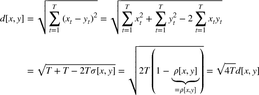
In other words, the distance d[x, y] is a linear multiple of the Euclidean distance between the vectors {X, Y} after z-standardization, hence it inherits the true-metric properties of the Euclidean distance.

Similarly, we can prove that descends to a true metric on the /2 quotient. In order to do that, we redefine , where sgn[.] is the sign operator, so that 0 ≤ ρ[x, y] = |ρ[x, y]|. Then,

16.A.2 Inverse Variance Allocation

Stage 3 (see Section 16.4.3) splits a weight in inverse proportion to the subset's variance. We now prove that such allocation is optimal when the covariance matrix is diagonal. Consider the standard quadratic optimization problem of size N,

with solution . For the characteristic vector a = 1_N, the solution is the minimum variance portfolio. If V is diagonal, . In the particular case of N = 2, , which is how stage 3 splits a weight between two bisections of a subset.

16.A.3 Reproducing the Numerical Example

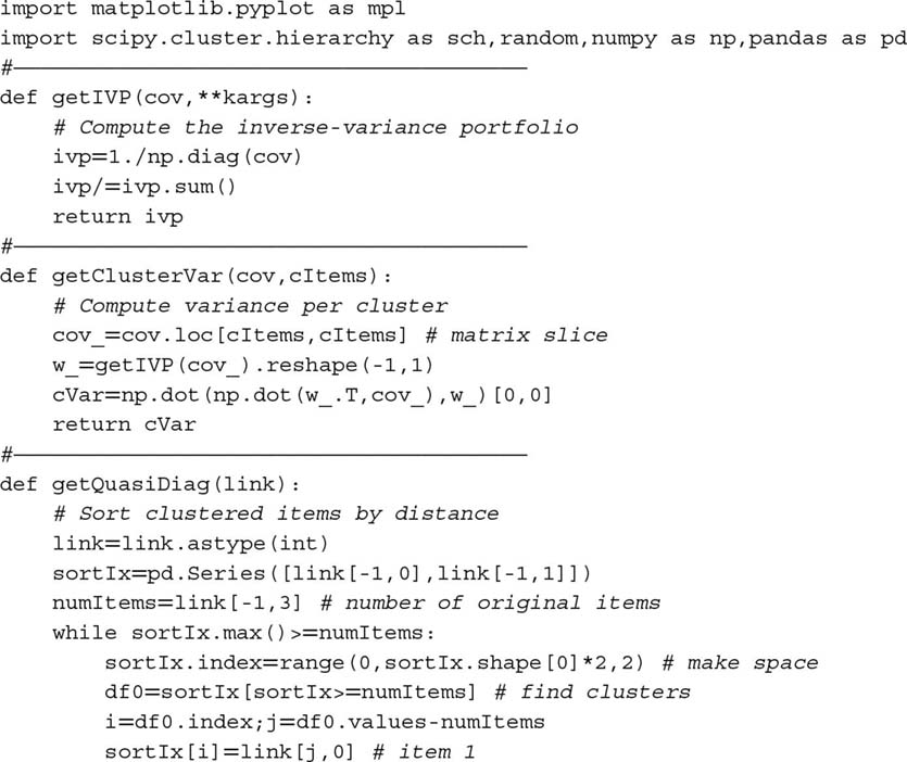
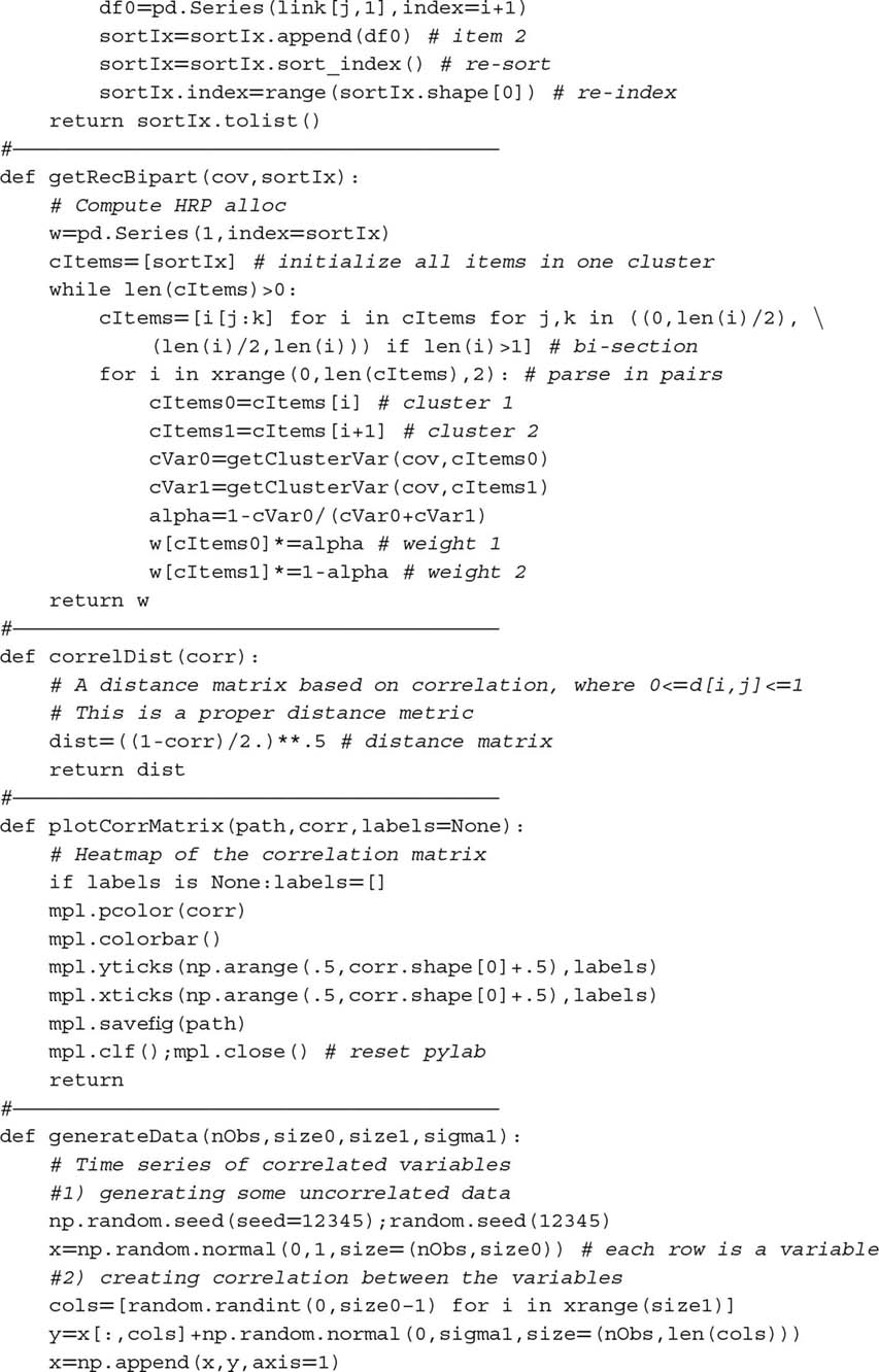
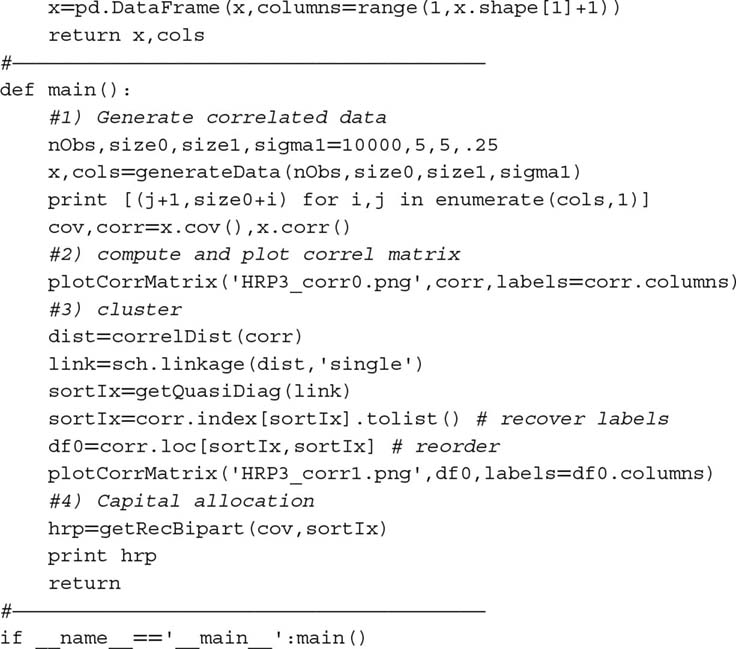
Snippet 16.4 can be used to reproduce our results and simulate additional numerical examples. Function generateData produces a matrix of time series where a number size0 of vectors are uncorrelated, and a number size1 of vectors are correlated. The reader can change the np.random.seed in generateData to run alternative examples and gain an intuition of how HRP works. Scipy's function linkage can be used to perform stage 1 (Section 16.4.1), function getQuasiDiag performs stage 2 (Section 16.4.2), and function getRecBipart carries out stage 3 (Section 16.4.3).

Snippet 16.4 Full implementation of the HRP algorithm

16.A.4 Reproducing the Monte Carlo Experiment

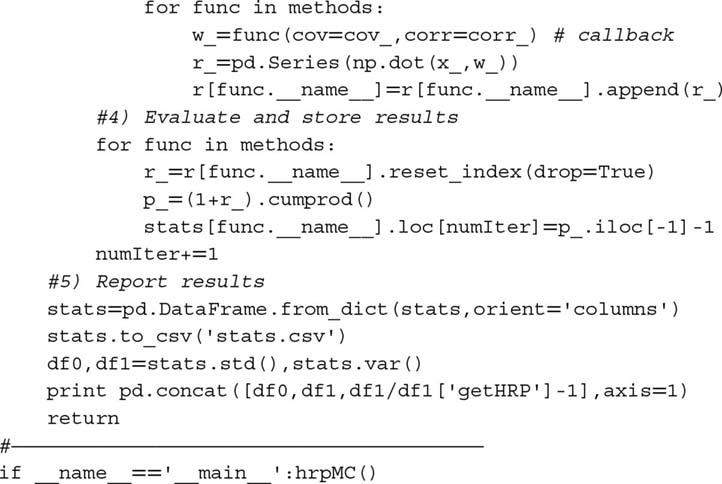
Snippet 16.5 implements Monte Carlo experiments on three allocation methods: HRP, CLA, and IVP. All libraries are standard except for HRP, which is provided in Appendix 16.A.3, and CLA, which can be found in Bailey and López de Prado [2013]. The subroutine generateData simulates the correlated data, with two types of random shocks: common to various investments and specific to a single investment. There are two shocks of each type, one positive and one negative. The variables for the experiments are set as arguments of hrpMC. They were chosen arbitrarily, and the user can experiment with alternative combinations.

Snippet 16.5 Monte Carlo experiment on HRP out-of-sample performance

Exercises

1. Given the PnL series on N investment strategies:

   1. Align them to the average frequency of their bets (e.g., weekly observations for strategies that trade on a weekly basis). Hint: This kind of data alignment is sometimes called “downsampling.”
   2. Compute the covariance of their returns, V.
   3. Identify the hierarchical clusters among the N strategies.
   4. Plot the clustered correlation matrix of the N strategies.

2. Using the clustered covariance matrix V from exercise 1:

   1. Compute the HRP allocations.
   2. Compute the CLA allocations.
   3. Compute the IVP allocations.

3. Using the covariance matrix V from exercise 1:

   1. Perform a spectral decomposition: VW = WΛ.
   2. Form an array ϵ by drawing N random numbers from a U[0, 1] distribution.
   3. Form an NxN matrix , where , n = 1, …, N.
   4. Compute .
   5. Repeat exercise 2, this time using as covariance matrix. What allocation method has been most impacted by the re-scaling of spectral variances?

4. How would you modify the HRP algorithm to produce allocations that add up to 0, where |w_n| ≤ 1, ∀n = 1, …, N?

5. Can you think of an easy way to incorporate expected returns in the HRP allocations?

References

1. Bailey, D. and M. López de Prado (2012): “Balanced baskets: A new approach to trading and hedging risks.” Journal of Investment Strategies, Vol. 1, No. 4, pp. 21–62. Available at http://ssrn.com/abstract=2066170.
2. Bailey, D. and M. López de Prado (2013): “An open-source implementation of the critical-line algorithm for portfolio optimization.” Algorithms, Vol. 6, No. 1, pp. 169–196. Available at http://ssrn.com/abstract=2197616.
3. Bailey, D., J. Borwein, M. López de Prado, and J. Zhu (2014) “Pseudo-mathematics and financial charlatanism: The effects of backtest overfitting on out-of-sample performance.” Notices of the American Mathematical Society, Vol. 61, No. 5, pp. 458–471. Available at http://ssrn.com/abstract=2308659.
4. Bailey, D. and M. López de Prado (2014): “The deflated Sharpe ratio: Correcting for selection bias, backtest overfitting and non-normality.” Journal of Portfolio Management, Vol. 40, No. 5, pp. 94–107.
5. Black, F. and R. Litterman (1992): “Global portfolio optimization.” Financial Analysts Journal, Vol. 48, pp. 28–43.
6. Brualdi, R. (2010): “The mutually beneficial relationship of graphs and matrices.” Conference Board of the Mathematical Sciences, Regional Conference Series in Mathematics, Nr. 115.
7. Calkin, N. and M. López de Prado (2014): “Stochastic flow diagrams.” Algorithmic Finance, Vol. 3, No. 1, pp. 21–42. Availble at http://ssrn.com/abstract=2379314.
8. Calkin, N. and M. López de Prado (2014): “The topology of macro financial flows: An application of stochastic flow diagrams.” Algorithmic Finance, Vol. 3, No. 1, pp. 43–85. Available at http://ssrn.com/abstract=2379319.
9. Clarke, R., H. De Silva, and S. Thorley (2002): “Portfolio constraints and the fundamental law of active management.” Financial Analysts Journal, Vol. 58, pp. 48–66.
10. De Miguel, V., L. Garlappi, and R. Uppal (2009): “Optimal versus naive diversification: How inefficient is the 1/N portfolio strategy?” Review of Financial Studies, Vol. 22, pp. 1915–1953.
11. Jurczenko, E. (2015): Risk-Based and Factor Investing, 1st ed. Elsevier Science.
12. Kolanovic, M., A. Lau, T. Lee, and R. Krishnamachari (2017): “Cross asset portfolios of tradable risk premia indices. Hierarchical risk parity: Enhancing returns at target volatility.” White paper, Global Quantitative & Derivatives Strategy. J.P. Morgan, April 26.
13. Kolm, P., R. Tutuncu and F. Fabozzi (2014): “60 years of portfolio optimization.” European Journal of Operational Research, Vol. 234, No. 2, pp. 356–371.
14. Kuhn, H. W. and A. W. Tucker (1951): “Nonlinear programming.” Proceedings of 2nd Berkeley Symposium. Berkeley, University of California Press, pp. 481–492.
15. Markowitz, H. (1952): “Portfolio selection.” Journal of Finance, Vol. 7, pp. 77–91.
16. Merton, R. (1976): “Option pricing when underlying stock returns are discontinuous.” Journal of Financial Economics, Vol. 3, pp. 125–144.
17. Michaud, R. (1998): Efficient Asset Allocation: A Practical Guide to Stock Portfolio Optimization and Asset Allocation, 1st ed. Harvard Business School Press.
18. Ledoit, O. and M. Wolf (2003): “Improved estimation of the covariance matrix of stock returns with an application to portfolio selection.” Journal of Empirical Finance, Vol. 10, No. 5, pp. 603–621.
19. Raffinot, T. (2017): “Hierarchical clustering based asset allocation.” Journal of Portfolio Management, forthcoming.
20. Rokach, L. and O. Maimon (2005): “Clustering methods,” in Rokach, L. and O. Maimon, eds., Data Mining and Knowledge Discovery Handbook. Springer, pp. 321–352.

Notes

1   A short version of this chapter appeared in the Journal of Portfolio Management, Vo1. 42, No. 4, pp. 59–69, Summer of 2016.

²   For additional metrics see:

• http://docs.scipy.org/doc/scipy/reference/generated/scipy.spatial.distance.pdist.html
• http://docs.scipy.org/doc/scipy-0.16.0/reference/generated/scipy.cluster.hierarchy.linkage.html