Chapter 4 – Amazon Neptun
e
Amazon Neptune Introduction
Amazon Neptune (Neptune) is a
graph database
engine and -- like RDS and Aurora -- a managed AWS database service.
26
Routine database admin tasks, typically performed by DBAs, such as provisioning hardware (i.e., scaling additional compute, memory, and storage resources), performing backups, applying software patches, detecting and reacting to failures, and recovering databases from backups are expedited and often automated by Neptune. Like Amazon Aurora, Neptune is also equipped with solid-state virtual storage facilities which are optimized for database workloads and deliberately engineered to significantly improve database performance, reliability, and availability. Neptune also promotes high availability by enabling automatic failover to read replicas and data replication across availability zones.
A Neptune graph database is fundamentally different from SQL-based relational database approaches, such as those engines supported by RDS. As previously noted, the data manipulation language (DML) for accessing most relational databases is some version or adaptation of SQL (e.g., an ANSI standard SQL version or a vendor specific SQL version).
In contrast, Neptune is categorized as a
NoSQL
(i.e., “Non SQL” or "Not Only SQL") database service which essentially means that Neptune provides a non-relational approach to managing, querying and manipulating data.
27
Instead of abiding by familiar relational concepts (i.e., tables with columns and foreign keys for implementing relationships), Neptune is based on
graph data structures
(i.e., vertices, edges, properties …. more on this later).
28
Also a Neptune graph database particularly appeals to applications with
highly connected
datasets and is accessed via well-known
graph query languages
(GQLs), such as
Gremlin
and
SPARQL
(
S
PARQL
P
rotocol
A
nd
R
DF
Q
uery
L
anguage).
29
Gremlin, developed by the
Apache TinkerPop
TM
open source project, provides a graph data query language as well as a virtual machine -- akin to a Java Virtual Machine (JVM) -- and is suitable for both OLTP and OLAP applications.
SPARQL is a semantic query language for accessing data stored in
RDF
(Resource Description Framework) format.
30
SPARQL is defined as a formal specification among the family of RDF recommendations from the W3C standards organization (World Wide Web Consortium). SPARQL supports a query syntax for traversing and navigating data in a graph database.
Regarding
highly connected
datasets, graph database engines and graph query languages are well-matched for applications that require navigating
complex network relationships
and also demand rapid results from queries. Complex network relationships typically include numerous, intersecting, many-to-many entity relationships such as those found in applications known as
recommender engines
.
6
Examples of such complex, many-to-many relationships include combinations of the following:
- A person can friend (or follow, or professionally connect to) many people … and each person can be friended (or followed or connected) by many other persons (e.g., social media for recommending friends, professional connections, persons to follow … as respectively for Facebook, LinkedIn, and Twitter).
- A person purchases many products or services … each product or service can be purchased by many people. For online retail recommending …
- Products or services
- Similar products or services
- Accessories of products purchased at the same time
- Products or services purchased by people who are friends, connections or live nearby
- A person visited many places (each with many attractions, hotels, restaurants, etc.) and each place has been visited by many people, friends, connections, neighbors -- for online travel recommendations.
Basic vocabulary of graph databases includes concepts such as vertices
(aka nodes
), edges
, and properties
as the basis for describing, storing and navigating data. These concepts are comparable to fundamental RDBMS concepts (i.e., table rows, foreign keys, columns) and data modeling concepts (i.e. entities, relationships, attributes):
-
Vertices (aka Nodes)
: Vertices or nodes are analogous to rows
in a relational table and to entity occurrences
using data modeling parlance. Vertices are assigned to one or more labels
-- comparable to a table name and table synonyms in a relational database -- for distinguishing node types (i.e., entities such as person, employee, location, product, asset, etc.).
-
Edges
:
Edges express an association or relationship between vertices (i.e., an edge is a connection that has a start node and an end node). In the RDBMS world, relationships
are implemented as foreign keys
and described as one-to-many relationships, many-to-many relationships, or one-to-one relationships in data models and data modeling tools.
-
Properties
:
Properties are comparable to RDBMS table columns
or attributes
of entities in a data model. Properties are stored as a collection of key-value pairs
(aka attribute–value pairs
) where the key
identifies (i.e., names or describes) the property and the value
is the data content of the property (e.g., where key
= ‘job_title’ and value
= ‘sales person’).31
The surprise is that properties apply to edges as well as vertices. Many key-value pairs can be defined for vertices and edges. Edges having properties is again reminiscent of the previously noted UML concept of an association class
where properties provide additional information about the edge and its association between its start and end vertices.32
Graph databases supporting these basic graph model concepts (i.e., vertices, edges, labels and properties) are called
labelled property graphs
(LPGs).
33
LPG concepts are comparable to relational vocabulary but the emphasis is somewhat different. The paradigm shift for GQLs is the prominence placed on edges. GQLs elevate edge relationships to a higher stature. Edges are explicitly named (i.e., labelled) components,
rather than being subtly inferred (as in the relational world) by foreign keys, creating indexes on foreign keys, and table joins for referencing and comparing values of foreign keys. The GQL focus is storing, searching and navigating edge interconnections between vertices. For many complex OLTP and OLAP applications, edges enable a direct linkage for more succinctly, intuitively, and efficiently traversing the linkages between vertices.
Gremlin Introduction
Unsurprisingly, the Gremlin query language syntax substantially differs from SQL. Specifically, Gremlin queries can concatenate a string of many retrieval operations -- referred to as
graph traversal steps
-- for successively navigating between vertices via edges.
34
For example, a Gremlin query can consist of a sequence of separate steps for traversing from vertex 1 (via a named edge) to vertex 2 -- and then concatenating additional steps for navigating from vertex 2 (via a differently named edge) to vertex 3, etc. The output of a step feeds into the subsequent step as its input. A single Gremlin query statement can traverse many vertices of different labels via different edge types with filters using properties of vertices or edges along the path.
Using
Gremlin console
commands, a brief summary of Gremlin’s rudimentary graph traversal steps for
C
reating,
R
eading,
U
pdating and
D
eleting graph data (i.e., fundamental CRUD data operations) -- in contrast to corresponding SQL statements -- is included as follows:
Gremlin Graph Traversal Steps -- Basics
-
addV
(Add Vertex): The Add Vertex step is analogous to a SQL INSERT statement for inserting a row into an RDBMS table. The addV
step adds a vertex to a graph and assigns one or more labels
indicating the associated type or types to which the vertex belongs. For example, multiple labels could connote synonyms or sub-type inheritance. Properties and property values are added to a vertex by chaining one or more property
(Add Property)
steps to an addV
step.
The following statement is a simple example for adding a vertex with an ID, name and date-of-birth properties:
g.addV
('person').property
(id, 'PER-0001').
property
('name','Random A. Person').property
('dob', '03/03/1995')
The following statement adds a person who is also an employee. Note that this includes two labels (perhaps connoting that an employee
is a sub-type of person
) with an additional property for the employee’s job title.
g.addV
(“person::employee”).property
(id, 'PER-0002').
property
('name',
'Random B. Person').
property
('dob', '04/04/1990').property
('title','sales person')
-
addE
(Add Edge): The
Add Edge step establishes a linkage between a starting vertex and an ending vertex. The addE
step assigns a label (e.g., friend, lives near, knows, purchased, etc.) for distinguishing different types of edges that can be established between vertices. The closest analogy to the relational world -- as
previously noted -- is the value of a column defined as foreign key implying a linkage to a row of another table (or the same table). The following statement is a simple example for adding an edge from a starting vertex to an ending vertex with a label “friend” indicating that a person is a friend of another person, and also includes a property for indicating the strength of the friendship:
g.addE
('friend').from(g.V('PER-0001')).to(g.V('PER-0002')).
property
('weight', 1.0)
-
Property
(Add Property): As noted in previous examples for the addV
and addE
steps, one or more properties can be defined for both vertices and edges. Different vertices or edges having the same label can flexibly include varying sets of properties -- unlike the structured relational approach whereby a
CREATE TABLE statement rigidly specifies columns that apply to all rows of a table. There is no analog in Gremlin to a CREATE TABLE statement. The property step can be used for conveniently adding properties to new or existing vertices and edges, and is also used for updating or appending values to previously defined properties.
-
Has:
The Has
step is used for filtering and is roughly analogous to a SQL SELECT statement for sifting rows from one or more RDBMS tables. But the Has
step applies to both vertices and edges. It is normally used for selecting vertices and edges based on property filters, somewhat comparable to using a WHERE clause in a SQL SELECT statement. There are many variations for the Has
step, several examples of which are included as follows:
-
Has (key, value)
: This option specifies a key and value. It selects vertices or edges whose property value equals the specified value.
-
Has (label, key, value)
: This option specifies a label, key and value. It selects the vertices or edges having the specified label, property and value.
-
hasLabel (label … )
: This option specifies one or more labels and selects the vertices or edges having at least one of the specified labels.
-
Has (key, predicate)
: This option specifies a key and a predicate (e.g., a comparison operator and value) for comparing the property value with the predicate. Examples of comparison operators include “eq” (equal to), “neq” (not equal to), “lt” (less than), “gt” (greater than), etc. This option selects vertices or edges for which the value of the specified property satisfies the predicate. A simple example of this option combined with the hasLabel option for counting employees who are sales people is included as follows:
g.V().hasLabel
('employee').has
('title',eq
('sales person')).count()
-
Drop:
The drop step -- roughly analogous to a SQL DELETE statement for removing rows from an RDBMS table -- can be used for deleting vertices, edges, or simply removing properties of vertices or edges. A simple example for removing the subset of 'sales person' vertices is included as follows:
g.V().has
('title','sales person').drop
(
)
The previous descriptions and examples of these basic steps represent the tip of the Gremlin iceberg (i.e., a small subset of the overall comprehensive assortment of graph traversal steps supported by Gremlin). These elementary steps are included here simply to provide a glimpse at Gremlin’s fundamental language concepts. A robust collection of many more steps and options are supported by Gremlin for allowing complex data transformations, filtering objects, calculating statistics, etc. Fortunately, abundant
documentation describing Gremlin
traversal steps (and providing copious examples with subtle nuances) is readily available online.
35
SPARQL Introduction
Unlike Gremlin, SPARQL as previously noted is targeted for data stored in
RDF
format and SPARQL’s syntax and semantics for querying and updating RDF data is more closely aligned with SQL. The RDF graph model (aka a
triple store
) stores linked data in the form of data
triples
derived from statements consisting of a
subject
+
predicate
+
object
. An RDF triple store is considered to be another type of graph database.
36
In an RDF graph, the subject and the object become vertices connected by an edge -- the predicate is an edge:
Triple Statement
➔
Subject (Vertex) + Predicate (Edge) + Object (Vertex)
Each triple statement links a subject (i.e., a vertex, typically a discrete entity occurrence such as an individual person, location, product, asset, etc.) via a predicate (edge) to another object (a vertex). In effect, the predicate names the relationship between the subject and object. The object is a discrete entity or can also be a simple literal value (e.g., a character string, date, integer, boolean, etc.) which also is stored as a vertex. Except for literals, objects in a triple statement can be the subject or object in other triple statements, thereby enabling graph traversal from subjects to objects as other subjects. Objects as literal values in essence are property values where the predicate is tantamount to being a property name as well as an edge (more about this later).
Examples of RDF triple statements, corresponding to examples of Gremlin graph traversal steps from in the previous section, are provided as follows:
g.addV
('person').property
(id, 'PER-0001').
property
('name','Random A. Person').property
('dob', '03/03/1995')
Corresponding RDF Triple Statements
…
- PER-0001
is a
person
- PER-0001
has name
‘Random A. Person’
- PER-0001
was born on
‘03/03/1995’
... Where “PER-0001” is a Subject … “is a”, “has name”, “was born on” are Predicates … “person” is an Object … ‘Random A. Person’ and ‘03/03/1995’ are literal Objects.
g.addV
(“person::employee”).property
(id, ‘PER-0002’).
property
(‘name’, 'Random B. Person').
property
(‘dob’,‘04/04/1990’).property
(‘title’,‘sales person’)
Corresponding RDF Triple Statements
…
- PER-0002
is an
employee
- employee
is a kind of
person
- PER-0002
has name
‘Random B. Person’
- PER-0002
was born on
‘04/04/1990’
- PER-0002
has job title
‘sales person’
… Where “PER-0002” is a Subject, “employee” is both an Object and Subject (i.e., in 2 separate statements) … “person” is an Object … “is an”, “is a kind of”, “has name”, “was born on”, “has job title” are Predicates … ‘Random B. Person’, ‘04/04/1990’, and ‘sales person’ are literal Objects.
Unlike Gremlin’s labelled property graphs where vertices and edges can each have many properties, RDF subjects and predicates do not have properties directly associated with them. In RDF, each property of a subject/vertex is implemented as a predicate/edge linking to an object as a literal value. As noted above, the predicate serves not only as an edge but is also analogous to a property name. So, in the previous triple statement ...
PER-0002 has job title ‘sales person’
…
the predicate “has job title” connects PER-0002 (subject) to the literal value ‘sales person’ (object = a character string) and, in essence, also suggests a property name (i.e., job_title). Each object, therefore, represents either some discrete entity occurrence (i.e., an individual person, place, product, event, thing, concept, etc.) or the value of some property of the subject. So … yes … property values can indeed be linked to a subject but, unlike an LPG, this results in the creation of another vertex and edge in the RDF graph. Clearly for implementing properties of subjects, an RDF graph is likely to contain many more vertices than those that would be required for an LPG.
But what about adding a property to an RDF predicate? Analogous to adding a property to an edge in an LPG, is it possible -- in some way -- to add information about an RDF predicate? Yes … but, sadly, the method for doing such is uncomfortably convoluted!
The RDF specification provides a technique called
RDF Reification
for adding information about an entire triple statement (e.g., the date the statement was made, the reason for the statement, the individual who made the statement, a rating or weight of the association, etc.).
37
In essence, adding information about a triple statement itself is tantamount to adding information about the predicate. In a nutshell -- without the gory details -- reification adds four
additional
triple statements (aka the “reification quad”) about the original statement itself. These additional statements amount to the inclusion of
metadata
within the RDF graph for describing the original statement. So, in this context,
the RDF graph not only contains application data (i.e., data about the problem domain), but now unfortunately also contains metadata (i.e., data about the data -- data about the statements themselves). This reification quad, therefore, sadly introduces substantially more vertices and edges than would be required for an LPG.
More specifically, the four additional statements, the reification quad, are summarized as follows:
-
A new triple statement defining the original statement itself:
-
Three additional statements for declaring its subject, predicate, and object.
Along with these four additional statements added to the RDF graph, yet another final
statement can now be created for achieving the ultimate goal of adding a property value for the original statement, i.e. for a linking another object or literal to the unique identifier for the original statement. Such complexity, in terms of the need for introducing additional vertices and edges -- for simply adding a property to a predicate -- is seemingly breath-taking in comparison to adding a property to an edge in an LPG. But that’s the bad news … Here perhaps is now the good news!
The SPARQL commands for creating, reading, updating, and deleting triple statements (CRUD) as previously indicated are somewhat comparable to SQL (i.e., SQL basic CRUD DML commands: INSERT, SELECT, UPDATE, DELETE). Data professionals (i.e., DBAs, database designers, applications developers, etc.) conversant in SQL are frequently quite comfortable if the need for transitioning to SPARQL arises. Several rudimentary SPARQL commands in comparison to SQL are briefly introduced as follows:
-
SELECT
: Comparable to the SQL SELECT statement for retrieving columns of rows from one or more relational tables, the SPARQL SELECT command queries and retrieves properties from one or more triples. Many key words are common to the SPARQL SELECT and SQL SELECT commands with comparable semantics (e.g., FROM, WHERE, GROUP BY, HAVING, UNION, DISTINCT, FILTER and many aggregate functions such as SUM, AVG, MIN, MAX, COUNT, etc.). There are of course many subtle differences. For example, the optional WHERE clause specifies search criteria in the form of one or more triple patterns
. A triple pattern is simply a triple statement where any of its components -- subject, predicate or object -- can be substituted with a variable for matching any vertex. Selected variables are returned in the query result. A FILTER key word can also be used to further constrain variable values. For example, a simple search of employees with job title “sales person” is provided as follows:
SELECT ?name
WHERE {
?employee prop:name ?name
?employee prop:jobtitle “sales person”
}
SPARQL variable names begin with a “?”, hence the variables ?employee, ?name, and ?jobtitle in the previous example.
-
INSERT DATA
: Comparable to the SQL INSERT statement for adding rows to a relational table, the SPARQL INSERT DATA command adds one or more triples to a specified or default RDF graph.
-
INSERT WHERE
: Based on search criteria specified in a WHERE clause, the INSERT WHERE command is a more powerful option for inserting one or more triples into an RDF graph. In this case, existing triples matching the specified search criteria are used as the basis for inserting new triples. Search results from the WHERE clause are combined with specified triple patterns for inserting new triples bound to the search results. A simple example is the need for inserting new triples for adding properties to subjects matched in the WHERE clause. The INSERT WHERE command can also be used for copying triples based on search criteria from a source graph to another graph.
-
DELETE DATA
: Comparable to the SQL DELETE statement for removing rows from a relational table, the SPARQL DELETE DATA command removes one or more specified triples from a specified or default RDF graph.
-
DELETE WHERE
: Based on search criteria specified in a WHERE clause, the DELETE WHERE command is a more powerful option for removing one or more triples from an RDF graph. In a manner similar to the INSERT WHERE command, triples matching the specified search criteria are used as the basis for removing existing triples. Search results from the WHERE clause are combined with one or more specified triple patterns for deleting existing triples bound to the search results. A simple example is the need for removing triples for properties predicated to subjects matched in the WHERE clause.
-
DELETE/INSERT WHERE
: SQL is endowed with an UPDATE statement
for directly modifying the content of existing rows in a relational table. Unlike SQL, SPARQL does not provide an analogous command for directly updating the content of existing triples. Instead, SPARQL provides the DELETE/INSERT statement -- which includes a WHERE clause -- for first removing existing triples and then inserting corresponding triples with revised information. Search results from the WHERE clause are combined with specified triple patterns for deleting existing triples and separate triple patterns for specifying updates.
Like the Gremlin introduction of the previous section, this brief introduction to SPARQL commands also represents the tip of the SPARQL iceberg (i.e., a small subset of the overall comprehensive assortment of key words and options supported by SPARQL). The command descriptions included herein simply provide a glimpse at SPARQL’s fundamental language concepts. Fortunately, abundant
documentation describing SPARQL
commands, examples, key words, options, and complex usage (e.g., joins between triples, outer joins, subqueries, etc.) is also readily available online.
38
Neptune Cluster
s
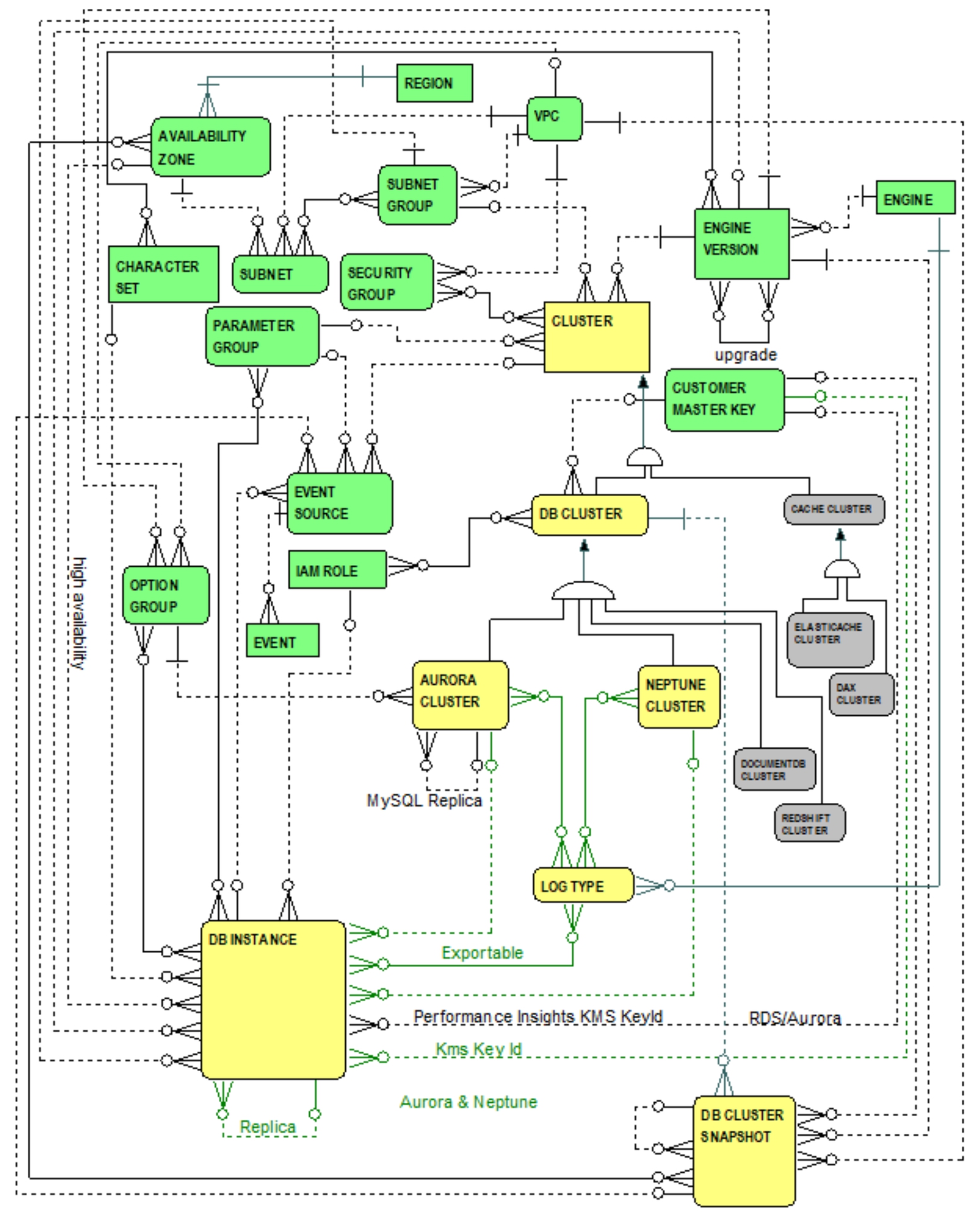
A Neptune cluster is very similar to an Aurora cluster. There are, however, some noteworthy differences that justify distinguishing Neptune clusters from Aurora clusters by establishing a new entity, the NEPTUNE CLUSTER entity. Figure 4.1 introduces entities and relationships focusing on Neptune cluster fundamental concepts.
Figure 4.1 Entities and Relationships … Neptune Fundamentals
Figure 4.1 highlights the NEPTUNE CLUSTER entity and reaffirms the explanation of the CLUSTER entity and its sub-type hierarchy in the previous chapter. Similar to Aurora, Neptune also enables the provisioning of a cluster of DB instances, consisting of
a primary DB instance and as many as 15 read replica DB instances. The NEPTUNE CLUSTER entity -- at the same level as the AURORA CLUSTER, DOCUMENTDB CLUSTER, and REDSHIFT CLUSTER entities -- is a sub-type of the DB CLUSTER entity. Each Neptune cluster is a kind of
DB cluster and, therefore, directly inherits attributes and relationships from the DB CLUSTER entity. Indirectly, it also enjoys inherited attributes and relationships from the CLUSTER entity.
More specifically, as a sub-type of the DB CLUSTER entity, a Neptune cluster (i.e., the graph
data maintained by all of its cluster DB instances) is optionally encrypted using a KMS customer master key, and benefits from one or more IAM roles enabling Neptune to access other AWS services on behalf of the Neptune cluster. From Figure 4.1 and as mentioned in the previous chapter, recall that a Neptune cluster -- as a kind of
DB cluster -- can be backed up by one or more DB cluster snapshots.
Common attributes inherited by the NEPTUNE CLUSTER entity from the DB CLUSTER entity include the following sample attributes noted as well in the previous chapter:
-
backup retention period:
The number of days that automatic backups are saved prior to being purged.
-
database name:
Identifies the name of the DB cluster’s initial database.
-
master username:
The master username for logging into the cluster’s DB instances.
-
storage encrypted:
Indicates whether or not the cluster’s data is encrypted.
Indirectly inherited from the CLUSTER entity, a Neptune cluster can serve as a source for event notifications and is associated with many security groups, a single subnet group, parameter group, and an engine version. This means that a cluster of Neptune DB instances is blessed with …
- A set of security groups for controlling access to Neptune cluster instances.
- A subnet group within whose subnets Neptune cluster instances can be launched.
- A single parameter group specifying parameters for configuring all Neptune cluster instances.
- A Neptune engine version for all cluster instances.
Common attributes indirectly inherited by the NEPTUNE CLUSTER entity from the CLUSTER entity include the sample attributes noted in the previous chapter:
-
cluster identifier:
A user-supplied cluster identifier.
-
cluster create time:
The time when the cluster was created.
-
status:
Indicates the current state of the cluster.
-
endpoint:
Specifies the cluster’s access information (i.e., DNS host name and port number) enabling applications to connect to the cluster.
-
preferred maintenance window:
Identifies the time period when maintenance activities (e.g., system upgrades) are preferred.
The one-to-many relationship from NEPTUNE CLUSTER entity to the DB INSTANCE entity indicates that each Neptune cluster is composed of one or more DB instances (i.e.,
all DB instances running the same Neptune engine version). One DB instance is primary and the remaining servers are read replicas. For example, via the Neptune console, when creating a Neptune cluster, a primary DB instance is automatically created for reading, writing and modifying data to the cluster volume. One or more replica DB instances -- possibly in separate availability zones for achieving high availability -- can be added to a Neptune cluster using the Neptune console, CLI, or API.
From 4.1, the optional one-to-many relationships from AURORA CLUSTER and NEPTUNE CLUSTER entities to the DB INSTANCE entity informally convey that each DB instance is exclusively either: 1) A member of an Aurora cluster, or 2) A member of a Neptune cluster, or 3) Neither -- simply a standalone RDS instance.
After a Neptune cluster is created, conventional tools and utilities (i.e., Gremlin, SPARQL, or Neptune utilities) running on client EC2 instances are used for connecting to graph databases. Examples of such utilities include the Gremlin Console, the
RDF4J
Console for SPARQL access,
39
and native Neptune endpoints enabling HTTP/REST queries for Gremlin and SPARQL.
Similar to Aurora, the one-to-many reflexive relationship from the DB INSTANCE entity to itself indicates that possibly many DB instances can serve as read replicas for the primary Neptune DB instance (i.e., a primary DB instance is synchronized to possibly many read replicas). Also similar to Aurora, the one-to-many relationship between CUSTOMER MASTER KEY and DB INSTANCE entities -- for encrypting DB instance data -- applies to Neptune DB instances. Also similar to Aurora, the many-to-many relationship between NEPTUNE CLUSTER and LOG TYPE entities affirms Neptune support for publishing log files to Amazon CloudWatch Logs.
In addition to previously described attributes inherited from its super-type hierarchy (i.e., foreign keys and other attributes inherited from the CLUSTER and DB CLUSTER entities), noteworthy examples of attributes pertinent to the NEPTUNE CLUSTER entity include:
-
multi AZ
: Indicates high availability in that DB instances are provisioned in more than one availability zone
.
-
preferred backup window:
If automatic backups are enabled, this indicates the time range (i.e., a user-defined daily time window) when automated backups are created.
-
earliest restorable time:
For restoring a cluster to a specific point-in-time, the earliest possible time in the past to the cluster can be recovered.
-
latest restorable time
: For restoring a cluster to a specific point-in-time, the latest possible time in the past the cluster can be recovered.
-
allocated storage
: Always set to 1 for Neptune indicating that Neptune storage size is not fixed but automatically scales as necessary.
Recall from the previous chapter that these immediately preceding attributes also apply to Aurora clusters. But these attributes are not applicable (as will be explored in subsequent chapters, e.g., Chapter 5 for DocumentDB) to other sub-types of the DB CLUSTER entity. These attributes, therefore, cannot be elevated to the DB CLUSTER entity thereby enabling inheritance by all of its sub-types
.
Aurora and Neptune cluster similarities suggest that perhaps Aurora and Neptune clusters might be generalized to yet another higher level of abstraction for hosting their common relationships and attributes (i.e., that the AURORA CLUSTER and NEPTUNE CLUSTER entities become sub-types of a new super-type entity beneath the DB CLUSTER super-type). The author, however, chose not to introduce this additional layer of complexity and defers exploring such (i.e., modifying Figure 4.1 to depict the suggested super-type) as an exercise for curious data modeling students. Recall from the explanation of a conceptual data model (CDM) and a more detailed logical data model (LDM) in the Introduction, that such an exercise might arguably be more appropriate and justifiable when evolving to an LDM from a CDM.
Neptune vs. Aurora Cluster Differences
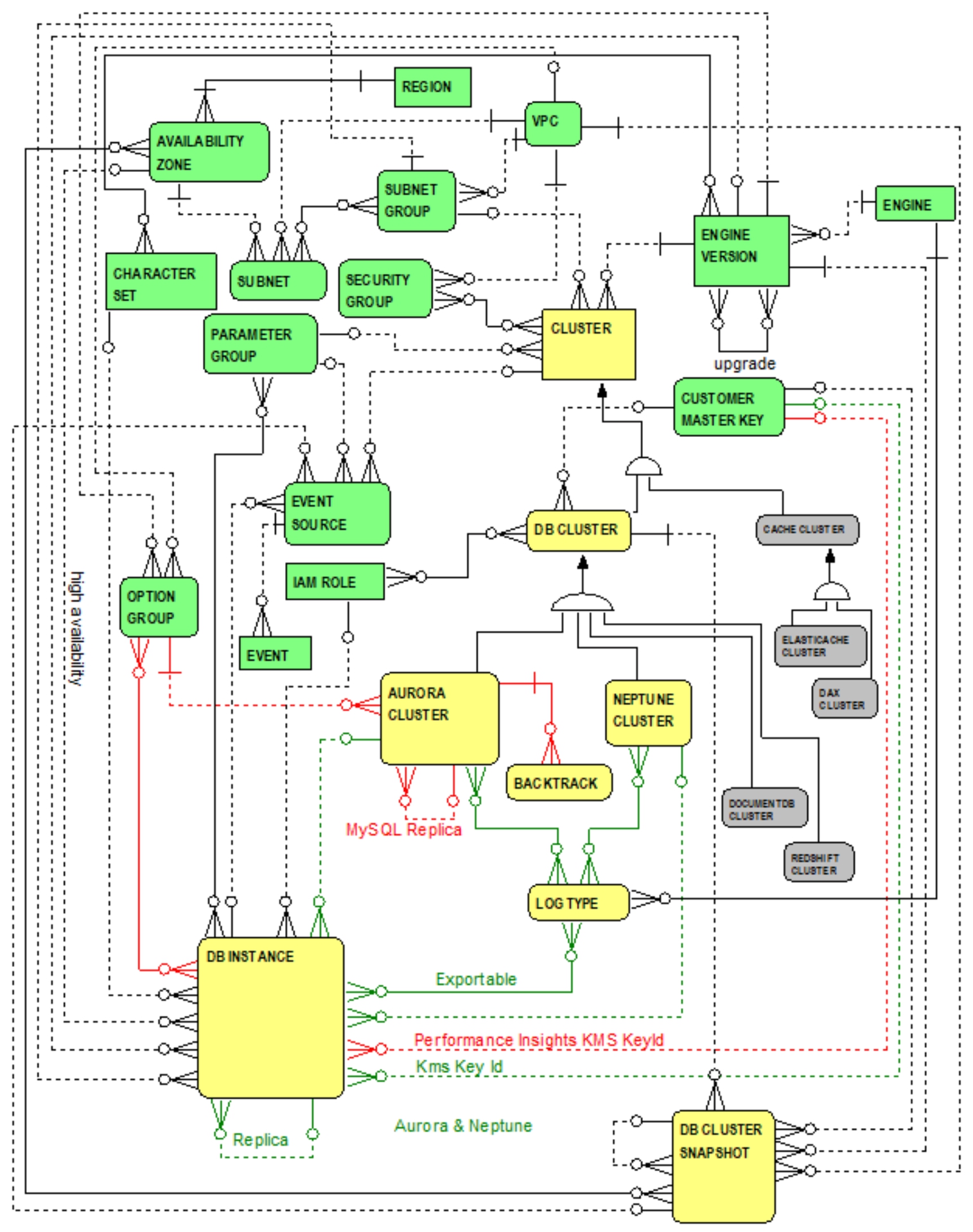
Clearly from the previous section, a Neptune cluster is similar to an Aurora cluster. Aurora clusters, however, exhibit several noteworthy curiosities in contrast with Neptune clusters which vindicate establishing the NEPTUNE CLUSTER entity as a justifiably distinct sub-type of the DB CLUSTER entity. Figure 4.2 highlights Aurora vs. Neptune major conceptual differences.
Figure 4.2 Entities and Relationships Highlighting Aurora vs. Neptune
From Figure 4.2, the following similarities (i.e., relationships highlighted in green), re-emphasized from the previous section for the reader’s convenience, are highlighted as follows:
- Each Aurora and Neptune cluster is a kind of
DB cluster (i.e., the AURORA
CLUSTER and NEPTUNE CLUSTER entities are sub-types of the DB CLUSTER entity) and as such enjoy all of the relationships and attributes directly inherited from their parent DB CLUSTER entity and indirectly inherited from their grandparent CLUSTER entity.
- Both Aurora and Neptune clusters each have a one-to-many relationship to the DB INSTANCE entity and share similar concepts and vocabulary. Each cluster is composed of one or more DB instances. One DB instance is primary and the remaining servers are read replicas.
- The reflexive relationship from the
DB INSTANCE entity to itself -- for read replicas -- applies to both Aurora and Neptune DB instances.
This indicates that possibly many DB instances that can serve as read replicas for a primary DB instance (i.e., a primary DB instance is synchronized to possibly many read replicas).
- Many-to-many relationships to the LOG TYPE entity highlight both Aurora and Neptune support for publishing log files to Amazon CloudWatch Logs.
- The one-to-many relationship between CUSTOMER MASTER KEY and DB INSTANCE entities -- for encrypting DB instance data -- applies to both Aurora and Neptune DB instances.
Figure 4.2 also highlights AURORA CLUSTER relationships to the BACKTRACK entity, OPTION GROUP entity, and its reflexive relationship (i.e., relationships highlighted in red). The differences? Unlike Aurora …
- Neptune does not support backtracking and serverless clusters.
- Neptune does not support the concept of option groups. Specifically, the one-to-many relationship from the OPTION GROUP entity to the AURORA CLUSTER entity -- reflecting the default option group applicable to all DB instances in an Aurora cluster -- is not applicable to Neptune clusters.
- Similarly, the many-to-many relationship between the DB INSTANCE and OPTION GROUP entities -- reflecting the option groups applicable to DB instances -- is not applicable to Neptune DB instances.
- The one-to-many relationship between
CUSTOMER MASTER KEY and DB INSTANCE entities -- labelled “Performance Insights KMS Key Id” for encrypting Performance Insights
metrics data -- is not applicable to Neptune DB instances.
- Neptune does not support cross-region replication. Specifically, the one-to-many reflexive relationship from AURORA CLUSTER entity to itself (highlighting support for cross-region replication for MySQL) is not applicable to Neptune clusters.
Lack of Neptune support for backtracking and serverless clusters means that the following attributes -- conveniently repeated here from the previous chapter -- are applicable to Aurora clusters but are not applicable
to Neptune clusters:
-
backtrack consumed change records
: The count of backtrack change records retained for the cluster.
-
backtrack window
: Amount of time in seconds for which a backtrack may be wanted, (e.g., a target backtrack window of 48 hours).
-
earliest backtrack time
: The earliest time for which a DB cluster backtrack can be requested (e.g., based on accumulated change records and available storage).
-
DB engine mode
: Indicates the engine mode (e.g., serverless, provisioned).
-
max capacity
: For a serverless cluster, the maximum capacity in terms of Aurora capacity units
(ACUs) expressing the peak capacity (i.e. compute and memory) to which Aurora can automatically expand.