Chapter 5

Scrub-a-Dub-Dub: Cleaning Data

IN THIS CHAPTER

Editing an imported workbook

Cleaning data with text functions

Keeping data clean with validation

No matter how hard you work to get data into Excel, the hard truth of the data analysis business is that in almost every case, the data that you start with — especially external data that you import from other programs — will be, at best, disorganized and, at worst, inconsistent and inaccurate. When data is messy, erratic, and wrong, data mavens describe it as dirty. Your job, should you decide to accept it, is to scrub that dirty data until it shines. Why? Because getting your data into a clean form makes it easier to work with, easier to organize, and easier to analyze. Best of all, Excel’s data-cleaning cup runneth over with tools and techniques that can help take the drudgery out of a necessary chore.

Editing Your Imported Workbook

I start this discussion with some basic workbook editing techniques. If you take a look at the workbook shown in Figure 5-1, you see that the data, although somewhat neatly formatted, suffers from quite a few problems:

• The data is a regular range, not an Excel table.
• The workbook has several blank rows and a blank column.
• The “numbers” you see in columns B, C, and F are actually text values. How can you tell? They’re left-aligned within their cells instead of being right-aligned, as is usual for numbers. Also, you see an error indicator in each cell, and when you click the error icon, Excel tells you that the cell contains a number formatted as text.
• The column are poorly sized for the data they contain. For example, columns A, B, C, and F are too wide, whereas column E is too narrow (which is why those pound signs (#) appear in some cells).

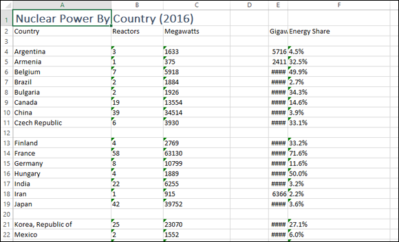
FIGURE 5-1: This worksheet needs a good scrubbing.

Alas, a dirty worksheet like the one shown in Figure 5-1 isn’t unusual. Fortunately, you can use several workbook-editing techniques to clean up a workbook. In the following sections, I give you a rundown of the most useful ones.

Deleting unnecessary columns

To delete unnecessary columns (these might be blank columns or columns that store data that you don't need), either click the column header to select the entire column and then choose Home ⇒ Delete, or right-click the column header and then click Delete.

You can also select a column by clicking any cell in the column and then pressing Ctrl+spacebar. You can select multiple columns for multiple deletions by holding down the Ctrl key and then individually selecting column headers.

Deleting unnecessary rows

To delete unnecessary rows (for example, blank rows or rows that contain unneeded data), either click the row header to select the entire row and then choose Home ⇒ Delete, or right-click the row header and then click Delete.

You can also select a row by clicking any cell in the row and then pressing Shift+spacebar. To select multiple rows for deletion, hold down the Ctrl key and then select the row header for each of the rows that you want to delete.

Resizing columns

To resize (that is, change the width of) a column so that its contents display clearly, you have four choices:

• Double-click the column header's right edge to size the column so that it’s just wide enough to fit its widest item. Handily, this also works if you select multiple columns and then double-click any one of their right edges.
• Select any cell in the column and then choose Home ⇒ Format ⇒ AutoFit Column Width. Excel widens the column just enough to fit its widest item.
• Select any cell in the column and then choose Home ⇒ Format ⇒ Column Width. In the Column Width dialog box that appears, enter the width you want to use and then click OK.
• Drag the right edge of the column header: Drag to the left for a narrower column, or drag to the right for a wider column.

Resizing rows

To resize (that is, change the height of) a row so that its contents appear fully without too much extra space above the content, you have four choices:

• Double-click the row header's bottom edge to size the row so that it’s just high enough to fit its tallest item. This also works if you select multiple rows and then double-click any one of their bottom edges.
• Select any cell in the row and then choose Home ⇒ Format ⇒ AutoFit Row Height. Excel resizes the row height just enough to fit its tallest item.
• Select any cell in the row and then choose Home ⇒ Format ⇒ Row Height. In the Row Height dialog box that appears, enter the height you want to use and then click OK.
• Drag the bottom edge of the row header: Drag down for a shorter row, or drag up for a taller row.

Erasing unneeded contents in a cell or range

To erase the contents of a cell or range that contains data you don’t need, select the worksheet cell or range and then choose Home ⇒ Clear ⇒ Clear All. Excel erases both the contents of the cells in the selected range and any formatting assigned to those cells.

Formatting numeric values

If you find that some of your data is in the wrong format (such as numbers displayed with text formatting), you have three techniques to use to apply the correct format for the data:

• Select the range you want to format, click the Number Format drop-down list on the Home tab, and then select the format you want to apply.
• Select the range you want to format and then select a predefined format in the Home tab’s Number group.
• Select the range you want to format, click the Number Format drop-down list on the Home tab, and then select More Number Formats. Excel displays the Format Cells dialog box with the Number tab displayed, as shown in Figure 5-2. Select a category and then select among the options (such as Decimal Places in the Number category) to specify the format you want to use. While you’re here. you can use the other tabs in this dialog box to change the formatting of the selected range. For example, select among the options from the Alignment tab to change the way the text and values are positioned in the cell; go to the Font tab to choose the font used for values and labels in the selected range; and go to the Border tab to assign cell borders to the selected range.

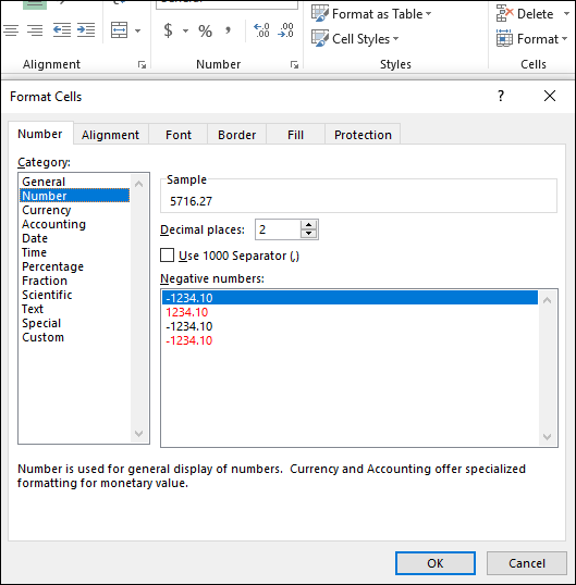
FIGURE 5-2: Format your numeric values here.

Copying worksheet data

To copy worksheet data, you have two choices:

• Select the data that you want to duplicate (which could be a single cell or range of cells) and then select Home ⇒ Copy (or press Ctrl+C). Select the cell that you want to use as the upper-left corner of the destination range and then select Home ⇒ Paste (or press Ctrl+V).
• Select the worksheet range that you want to copy, hold down the Ctrl key, and then drag the range border to the destination range where you want the copy to appear.

Moving worksheet data

To move worksheet data, you have two techniques to choose from:

• Select the range you want to move (a single cell or range of cells) and then choose Home ⇒ Cut (or press Ctrl+X). Select the cell that you want to use as the upper-left corner of the destination range and then choose Home ⇒ Paste (or press Ctrl+V).
• Select the worksheet range that you want to move and then drag the range border to the new position where you want the data to appear.

Replacing data in fields

Here are some common causes of crud in an imported worksheet:

• Extraneous characters
• Repeated characters
• Misspelled words
• Inconsistent spellings of certain words
• Abbreviations or acronyms instead of full words

Sure, you could trudge through the entire worksheet and manually fix all these annoying glitches, but who has time for that? Instead, let Excel do the heavy lifting with its irreplaceable Replace command. With Replace, you tell it what text you don’t want, tell it what text to use instead, and then let it rip. The result? Cleaner data without so much as a scrub brush in sight.

To use Replace, choose Home ⇒ Find & Select ⇒ Replace to open the Find and Replace dialog box with the Replace tab displayed, as shown in Figure 5-3. Enter the incorrect text that you want to find in the Find What text box and then enter the correct text in the Replace With text box. Now you have two ways to proceed:

• Click Find Next to find the next instance of the Find What text. If you want to change this instance, click Replace; otherwise, click Find Next. Repeat until you’ve run through all the instances.
• If you’re absolutely certain that you want to replace every last instance of the Find What text with the Replace With text, click the Replace All button to make all the changes at one time.

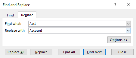
FIGURE 5-3: Fix funky data with Excel’s Replace feature.

Cleaning Data with Text Functions

One of the common problems with data that you import is that your text labels aren't quite right. For example, you might find yourself with the city, state, and ZIP code information that's part of an address stored in a single cell rather than in three separate cells. Or you might find that same information stored in three separate cells when you want the data stored in a single cell. You might also find that pieces of information that you want stored as labels instead are stored as values, and vice versa.

I mentioned in the previous section that you can use Excel’s Replace feature to handle some data-cleaning chores, but Excel also offers lots of useful worksheet functions that can give you much more control over how you scrub your data. The next few sections take you through these functions and explain how they can make your data-cleaning chores go much faster and easier.

For each of the text functions that follow, I’ve set up an example worksheet in the Chapter05.xlsx file that accompanies this chapter. See the Introduction to learn how to access this file. Also, the functions that follow all require one or more text arguments. Rather than repeat what text means each time, I summarize the possibilities here:

• A string literal — that is, some text surrounded by double quotation marks (such as "Hello World!")
• A reference to a cell that contains text
• A function that returns a text result

The CLEAN function

You use the CLEAN function to remove nonprintable characters from the text. For example, if the text in a column is displaying characters that appear as solid blocks or weird symbols, it means that Excel doesn't recognize those characters.

A more common scenario is imported data where one or more cells contain multiple lines of text, which means that the text includes one or more line feeds or carriage returns. CLEAN can expunge the line feeds and carriage returns, making the data display on a single line.

You can apply the CLEAN function to each cell in the column, which enables you to store the cleaned-up text in a new column that you can work with instead of the original.

The CLEAN function uses the following syntax:

CLEAN(text)

For example, to clean the text stored in cell A2, use the following syntax:

CLEAN(A2)

The CONCAT function

The CONCAT function joins two or more chunks of text into a single string. This is extremely useful if a particular bit of data (such as a name) is split over multiple columns (such as separate first name and last name columns).

The CONCAT function uses the following syntax:

CONCAT(text1, text2, text3,…)

The text1, text2, text3, and so on arguments are the chunks of text that you want to combine into a single string. For example, if your data displays first names in column A and last names in column B, you can add a new column named Full Name and use CONCAT to populate the new column with each first name and last name joined together, separated by a space. Here's an example:

CONCAT(A1, " ", B1)

This tells Excel to take the text from cell A1, tack on a space, and then add the text from cell B1. If A1 contains “Paul” and B1 contains “McFedries,” the CONCAT function returns the following string:

Paul McFedries

Having said all that, I’m also duty-bound to point out that no one ever uses the CONCAT function. Why not? Because Excel offers an easier method to join strings: the concatenation operator (&). When you insert this operator between two strings, Excel joins them together, like so:

A1 & " " & B1

I talk about an even more powerful way to join strings in “The TEXTJOIN function” section, later in this chapter, which covers Excel’s new TEXTJOIN function.

The EXACT function

The EXACT function compares two strings. If the two strings are exactly the same, the EXACT function returns the logical value TRUE. If the two strings differ in any way, the EXACT function returns the logical value FALSE. The EXACT function is case sensitive. For example, Redmond spelled with a capital R differs from redmond spelled with a lowercase r.

The EXACT function uses the following syntax:

EXACT(text1,text2)

The text1 and text2 arguments are the strings that you want to compare. For example, to check whether the two strings "Redmond" and "redmond" are the same, use the following:

EXACT("Redmond","redmond")

This function returns the logical value FALSE because these two strings don't match exactly. One begins with an uppercase R and the other begins with a lowercase r.

The FIND function

The FIND function finds the starting character position of one string within another string. For example, if you have a column of full names (first and last), you might want to know where the space occurs in each name (which would be handy when you want to write a formula that splits the names). The FIND function handles that chore with no problem.

The FIND function uses the following syntax:

FIND(find_text,within_text,[start_num])

The find_text argument is the text that you're looking for. The within_text argument identifies where or for what you’re searching. The optional start_num argument tells Excel at what point within the string it should begin its search. For example, to find at what point the two-letter state abbreviation WA begins in the string Redmond WA 98052, use the following:

FIND("WA","Redmond WA 98052",1)

The function returns the value 9 because WA begins at the ninth position (because spaces are counted).

As another example, suppose you have the text “Paul McFedries” in cell A2. Here's an expression that returns the location of the space (5, in this case):

FIND(" ", A2)

The start_num function argument is optional. If you omit this argument, Excel begins searching at the beginning of the string.

FIND runs a case-sensitive search, meaning that FIND("Sales ", A2 ) will return a number if A2 contains “Annual Sales” or “Sales Representative”, but it will return a #VALUE! error if A2 contains “The sales team” or “salesperson.” To locate text within a string without having to worry about case, use the SEARCH function that I describe later in this chapter (see the section “The SEARCH function”).

The LEFT function

The LEFT function returns a specified number of characters from the left end of a string. The function uses the following syntax:

LEFT(text,num_chars)

The text argument either supplies the string or references the cell holding the string. The optional num_chars argument tells Excel how many characters to grab.

For example, to grab the leftmost seven characters from the string Redmond WA, use the following formula:

LEFT("Redmond WA",7)

The function returns the text Redmond.

On a more practical note, suppose you have a column of full names and you want to extract the first name. To do this, first use the FIND function to locate the space in the full name; then use the LEFT function to extract up to, but not including, the location of the space. For example, suppose you have the text “Paul McFedries” in cell A2. Here's an expression that extracts the first name from this text:

LEFT(A2, FIND(" ", A2) – 1)

The LEN function

The LEN function counts the number of characters in a string. The function uses the following syntax:

LEN(text)

The text argument either supplies the string that you want to measure or references the cell holding the string. For example, to measure the length of the string in cell I81, use the following formula:

LEN(I81)

If cell I81 holds the string Semper fidelis, the function returns the value 14. Spaces are counted as characters, too.

The LOWER function

Many external databases return all-uppercase data, which is a pain. If an all-uppercase column should really be all-lowercase, use the LOWER function, which returns an all-lowercase version of a string. The function uses the following syntax:

LOWER(text)

The text argument either supplies the string that you want to convert or references the cell holding the string. For example, to convert the string PROFESSIONAL to professional, use the following formula:

LOWER("PROFESSIONAL")

The function returns professional.

The MID function

The MID function returns a chunk of text from inside (that is, not necessarily from the beginning or the end) of a string. The function uses the following syntax:

MID(text, start_num, num_char)

The start_num argument tells Excel where the text fragment starts that you want to grab. The num_char argument tells Excel how many characters long the text fragment is. For example, to grab the text fragment tac from the string tic tac toe, use the following formula:

=MID("tic tac toe",5,3)

In many cases, you don't know the starting point of the string that you want to extract because the text prior to that point isn’t a fixed length. For example, here are some part numbers that you might have imported from a database:

LDW-2125-X52
MP-9790-C78
PNH-7793-W40
SA-8703-I16
RB-3024-Z87
N-4191-W23

Suppose you want to extract the four digits that appear between the hyphens (-). How do you do that when the string before the first hyphen is anywhere from one to three characters long?

For starters, use the FIND function to locate the first hyphen, and then add 1 to get the starting point of the four-digit numeric value. Here’s expression to use if the text is in cell A2:

FIND("-", A2) + 1

You can then plug this expression into your MID function:

MID(A2, FIND("-", A2) + 1, 4)

For the first example string, this expression return 2125.

The NUMBERVALUE function

The NUMBERVALUE function converts digits formatted as a string to a true numeric value. Here’s the syntax:

NUMBERVALUE(text, decimal_separator, group_separator)

Here, decimal_separator is the character used in the string to separate the decimal portion of the number, and group_separator is the character used in the string to separate the groups (that is, thousands, millions, and so on) of the number.

For example, the formula I use in the previous section to extract four digits from within a string returns those digits as a string instead of a number. Assuming that one such string resides in cell B2, you use the following expression to convert it to a number:

NUMBERVALUE(B2)

As another example, suppose your imported data includes the following values as strings:

71.970,53
3.479,39
68.774,80
9.205,36
88.852,73

To convert these strings to numbers, you use the following version of NUMBERVALUE (assuming that the first string is in B2):

NUMBERVALUE(B2, ",", ".")

This tells Excel to treat the comma (,) as the decimal separator and the period (.) as the group separator . For the first string, this function returns the numeric value 71970.53.

The PROPER function

The PROPER function capitalizes the first letter of every word in a string. The function uses the following syntax:

PROPER(text)

For example, to capitalize the initial letters in the string SALES REPRESENTATIVE , use the following formula:

PROPER("SALES REPRESENTATIVE")

The function returns the string Sales Representative.

The REPLACE function

The REPLACE function replaces a portion of a string with new text. The function uses the following syntax:

REPLACE(old_text, start_num, num_chars, new_text)

The old_text argument, which is case sensitive, either supplies the string from which you grab some text fragment or references the cell holding the string. The start_num argument, which is the starting position, tells Excel where the text starts that you want to replace. The num_chars argument tells Excel the length of the text fragment (how many characters) that you want to replace. The new_text argument tells Excel what new text you want to use to replace the old text.

For example, to replace the string man with the string Representative in the string Salesman, use the following expression:

REPLACE("Salesman",6,3," Representative")

The function returns the string Sales Representative.

The RIGHT function

The RIGHT function returns a specified number of characters from the end of a string. The function uses the following syntax:

RIGHT(text,num_chars)

The num_chars argument tells Excel how many characters to grab from the end of text.

For example, to get the rightmost two characters from the string Redmond WA, use the following expression:

RIGHT("Redmond WA",2)

The function returns the text WA.

As another example, suppose you have a column of full names — that is, a first name and last name separated by a space — and you want to extract the last name. Okay, begin by using FIND to locate the space in the full name, and then use the RIGHT function to extract everything after the location of the space. Hmm, how many characters is that? It's the total length of the string (as given by the LEN function) minus the location of the space:

LEN(text) – FIND(" ", text)

Now you plug this expression into the RIGHT function as the num_chars argument. For example, suppose you have the text “Paul McFedries” in cell A2. Here’s an expression that extracts the last name from this text:

RIGHT(A2, LEN(A2) - FIND(" ", A2))

The SEARCH function

The SEARCH function performs a case-insensitive search to return the starting position of a specified string within a larger string. The function uses the following syntax:

SEARCH(find_text,within_text,start_num)

The find_text argument tells Excel what string fragment you're looking for. The within_text argument tells Excel what string you want to search. The optional start_num argument tells Excel where to start its search. (If you omit start_num, Excel starts the search at the beginning of within_text.)

For example, to identify the position at which the text fragment Churchill starts in the string Mr.  Churchill, use the following formula:

SEARCH("Churchill","Mr. Churchill",1)

The function returns the value 5.

The SUBSTITUTE function

The SUBSTITUTE function replaces occurrences of text in a string. The function uses the following syntax:

SUBSTITUTE(text,old_text,new_text,instance_num)

The old_text argument identifies the to-be-replaced text fragment; new_text supplies the new replacement text; and the optional instance_num argument specifies which instance of old_text you want replaced. (If you omit this argument, Excel replaces all the instances.)

As an example of how the SUBSTITUTE function works, suppose your imported data comes with a phone number column in which the numbers use the following format:

123 555 6789

Assuming that one such string is in cell A2, here's a SUBSTITUTE expression that replaces all the spaces with dashes:

SUBSTITUTE(A2, " ", "-")

The TEXT function

The TEXT function formats a value and then returns the value as text. The function uses the following syntax:

TEXT(value,format_text)

The value argument is the value that you want formatted and returned as text. The format_text argument is a string that shows the currency symbol and placement, commas, and decimal places that you want. For example, the formula

=TEXT(1234.5678,"$##,###.00")

returns the text $1,234.57.

The TEXTJOIN function

The TEXTJOIN function combines two or more strings into a single string with a specified character — called the delimiter — between each of the original strings. The function uses the following syntax:

TEXTJOIN(delimiter,ignore_empty, text1, text2,…))

The delimiter argument is the character you want placed between the concatenated strings (or, if you want everything smashed together without anything in between, using ""). The ignore_empty argument tells Excel whether it should ignore empty cells when joining the string; the default is TRUE; text1, text2, and so on are the strings you want to join.

For example, suppose you imported some data that includes separate fields for three types of code: Manufacturer, Category, and Location. Suppose further that you can generate the values of a Part Number field by combining these three codes into a single string, with the codes separated by hyphens (-). If the three codes are in cells A2, B2, and C2, here's a TEXTJOIN expression that generates a part number

=TEXTJOIN("-", TRUE, A2, B2, C2)

Figure 5-4 shows an example of this expression in action.

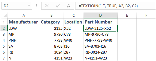
FIGURE 5-4: The TEXTJOIN function doing its thing.

The TRIM function

Some of the biggest causes of untidiness in imported data are extra characters added to some or all of the cells. For example, many cells come with extra spaces before, after, and even within the cell value. Other cells might have line breaks (caused by extraneous line feed or carriage return characters) or tabs.

The aptly named TRIM function removes extra spaces, line feeds, carriage returns, and tabs from a string. The function uses the following syntax:

TRIM(text)

For example, to trim the text stored in cell A2, use the following syntax:

TRIM(A2)

The UPPER function

The UPPER function returns an all-uppercase version of a string. The function uses the following syntax:

UPPER(text)

For example, to convert the string professional to PROFESSIONAL, you can use the following formula:

UPPER("professional")

The function returns the string PROFESSIONAL.

The VALUE function

The VALUE function converts a string that looks like a numeric value to an actual number. The function uses the following syntax:

VALUE(text)

For example, to convert the string $123,456.78 — assume that this isn't a numeric value but a string — you use the following expression:

VALUE("$123,456.78")

The function returns the numeric value 123456.78.

Converting text function formulas to text

When you’re using text functions to clean up imported data, the most common technique is to start a new column beside the data and then create a formula that uses a text function to convert the first cell of the imported data into the format you want. You then fill that formula down the column to get cleaned-up versions of all the cells.

The aforementioned technique works like a charm, except for one inconvenient fact: Your cleaned-up versions appear as formula results instead of plain text or numbers. That won’t be inconvenient for long because you can convert those formulas to the strings and numbers that they return. Here’s how:

1. Select the worksheet range that holds the formulas.
2. Choose Home ⇒ Copy.

3. Choose Home ⇒ Paste ⇒ Paste Values.

   Because you left the formula range selected, the paste replaces the formulas with the values they returned.

Using Validation to Keep Data Clean

One useful command related to this business of keeping your data clean is the Data Validation command. Use this command to describe what information can be entered into a cell. The command also enables you to supply messages that give data input information and error messages that attempt to help someone correct data-entry errors.

To use Data Validation, follow these steps:

1. Select the worksheet range where the to-be-validated data will go.

   You can do this by dragging your mouse or by using the navigation keys.

2. Choose Data ⇒ Data Validation.

   Excel displays the Data Validation dialog box, as shown in Figure 5-5.

3. On the Settings tab of the Data Validation dialog box, use the controls in the Validation Criteria area to describe what is valid data.

   Select options from the Allow drop-down list box, for example, to supply what types of information can go into the range: whole numbers, decimal numbers, values from the list, valid dates, valid times, text of a particular length, and so on.

   Select options from the Data drop-down list box to further define your validation criteria. The Data drop-down list box provides several comparisons that can be made as part of the validation: between, not between, equal to, not equal to, greater than, and so on.

   Refine the validation criteria, if necessary, by selecting from any of the other drop-down list boxes available. Note: The other validation criteria options depend on what you enter into the Allow and Data drop-down list boxes. For example, as shown in Figure 5-5, if you indicate that you want to allow only whole numbers between a particular range of minimum and maximum values, Excel provides Minimum and Maximum text boxes for you to enter or define the range. However, if you select other entries from the Allow or Data drop-down list boxes, you see other text boxes appearing on the Settings tab. In other words, Excel customizes the Settings tab depending on the kind of validation criteria that you define.

4. Fine-tune the validation.

   After you describe the validation criteria, either select or deselect (clear) the Ignore Blank check box to indicate whether blank cells are allowed.

5. (Optional) Consider expanding the scope of the data validation.

   Select the Apply These Changes to All Other Cells with the Same Settings check box to indicate whether the validation criteria should be expanded to other similar cells.

   Click the Clear All button, and Excel clears (removes) the validation criteria.

6. Provide an input message from the Input Message tab of the Data Validation dialog box.

   The Input Message tab, as shown in Figure 5-6, enables you to tell Excel to display a small message when a cell with specified data validation is selected. To create the input message, you enter a title for the message into the Title text box and message text into the Input Message text box. Make sure that the Show Input Message When Cell Is Selected check box is selected. Look at Figure 5-7 to see how the Input Message entered in Figure 5-6 looks in the workbook.

7. Provide an error message from the Error Alert tab of the Data Validation dialog box (see Figure 5-8).

   You can also supply an error message that Excel displays when someone attempts to enter invalid data. To create an error message, first verify that the Show Error Alert After Invalid Data Is Entered check box is selected. Then use the Style drop-down list box to select what Excel should do when it encounters invalid data: Stop the data entry on the user without the incorrect data entry, or simply display an informational message after the data has been entered.

   Just as you do when creating an input message, enter the error message title into the Title text box. Then enter the full text of the error message into the Error Message text box. In Figure 5-8, you can see a completed Error Alert tab. Check out Figure 5-9 for how the error message appears after a user enters invalid data.

   Curious about the options in the Style drop-down list box (as shown in Figure 5-8)? The style of the error alert determines what icon and command buttons the error message presents when someone attempts to enter bad data. If the error style is Stop, the error message box displays Retry and Cancel command buttons. If the error style is Warning, the error message box displays Yes, No, and Cancel command buttons. If the error style is Informational, the error message box displays OK and Cancel command buttons.

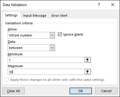
FIGURE 5-5: Keep data clean with the Data Validation dialog box.

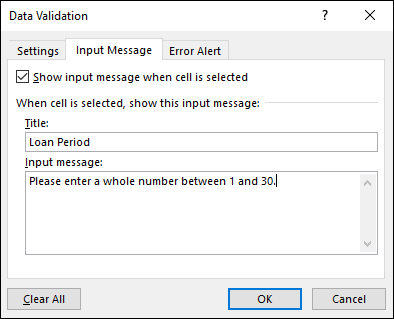
FIGURE 5-6: Create a data entry instruction message.

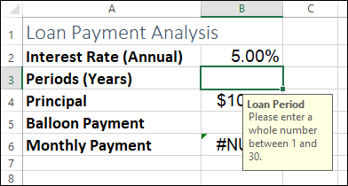
FIGURE 5-7: When the user selects the cell, Excel displays the message.

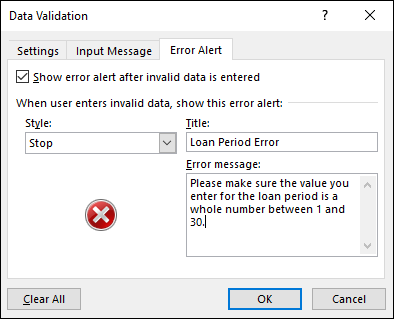
FIGURE 5-8: Create an annoying data-entry error message.

FIGURE 5-9: If the user enters invalid data, the error message rears its head.