Chapter 11

Analyzing Data with Statistics

IN THIS CHAPTER

Learning the countless ways to count things in Excel

Calculating the mean, median, mode, and other averages

Figuring out a value’s rank in relation to the rest of the data

Grouping your data into a frequency distribution

Messing around with statistical powerhouses such as standard deviation and correlation

Excel is a statistics powerhouse that boasts more than 100 statistical worksheet functions. That’s great if you’re a statistician, but do you really need all that stats muscle if you’re just doing basic data analysis? You’ll no doubt be relieved to hear that the answer is a resounding “No!” Most of Excel’s statistical features redefine the word esoteric. Believe me when I tell you that you can safely do without Excel features such as cumulative beta probability density and Fourier analysis. I merrily skip over those features and many more in this chapter as I focus on Excel’s most important and most useful statistical methods, including calculating the average, rank, largest and smallest values, variance, standard deviation, and correlation. Will it be fun? No, don’t be silly. Will it be useful? You bet.

Counting Things

The simplest statistical method you can apply to your data is to count the items in that data set. Of course, Excel being Excel, just because counting things is simple, counting things in Excel is complex because the program offers — count ’em — four functions related to counting items a worksheet: COUNT, COUNTA, COUNTBLANK, and COUNTIF. As if that’s not enough, Excel also provides two extra functions — PERMUT and COMBIN — that handle permutations and combinations, respectively.

Counting numbers

The COUNT function tallies the number of cells within a specified range that hold numeric values. That is, COUNT ignores cells that contain text (including numbers values that are formatted as text), that contain the logical values TRUE or FALSE, and that are empty. (It's worth noting that COUNT does include cells that contain dates or times, because Excel treats those data types as numbers.) Here’s the syntax:

=COUNT(value1[, value2, …])

Here, value1, value2, and so on are cell or range references. For example, to use the COUNT function to return how many numeric values are in the range B3:B12 in the worksheet shown in Figure 11-1, use the following formula:

=COUNT(B3:B12)

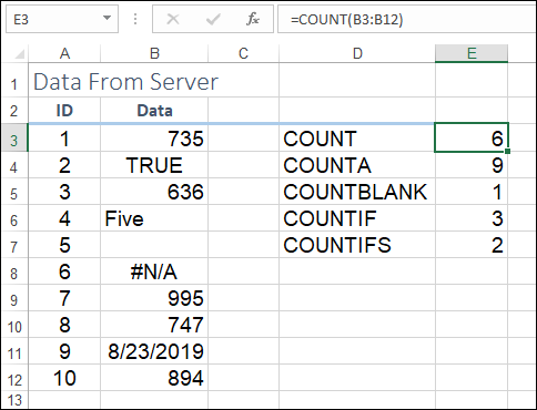
FIGURE 11-1: COUNT returns the tally of the numeric values in a range.

As shown in cell E3, COUNT returns 6 (five numbers plus one date).

Counting nonempty cells

The COUNTA function counts the number of cells within a specified range that are nonempty. It doesn't matter what data types the cells use — they could be numbers, dates, times, logical values, or text. As long as a cell contains something, it gets included in the COUNT A total. Here’s the COUNTA syntax:

=COUNTA(value1[, value2, …])

Here, value1, value2, and so on are cell or range references. For example, to use COUNTA to calculate how many nonempty values are in the range B3:B12 in the worksheet shown earlier in Figure 11-1, use the following formula:

=COUNTA(B3:B12)

As you can see in cell E4 in Figure 11-1, COUNTA returns the value 9.

Counting empty cells

The COUNTBLANK function is the functional opposite of COUNTA in that it counts the number of cells within a specified range that are empty. Here's the COUNTBLANK syntax:

=COUNTBLANK(value1[, value2, …])

Here, value1, value2, and so on are cell or range references. For example, to use COUNTBLANK to return how many empty values are in the range B3:B12 in the worksheet shown earlier in Figure 11-1, use the following formula:

=COUNTBLANK(B3:B12)

As you can see in cell E5 in Figure 11-1, COUNTBLANK returns the value 1.

Counting cells that match criteria

The COUNT, COUNTA, and COUNTBLANK functions count numbers, nonempty cells, and empty cells, respectively, so they have, in a sense, built-in criteria for what they count and what they ignore. If you have your own criteria for what should get counted and what shouldn't, you can turn to the COUNTIF function to apply that condition. Here’s the syntax:

=COUNTIF(range, criteria)

Here, range is the worksheet range over which you want to count cells, and criteria is a logical expression, enclosed in quotation marks, that specifies which cells in the range should be counted.

For example, looking back at the range B3:B12 in Figure 11-1, suppose you want to know how many cells contain a value greater than 800. Here's a formula that’ll get the job done:

=COUNTIF(B3:B12,">800")

As you can see in cell E6 in Figure 11-1, this formula returns the value 3. (There are two numbers greater than 800, plus the date value is equal to 43700, so it also meets the criteria.)

You can use any of the standard logical operators when building your criteria expression: Use the < operator for a less-than comparison; the <= operator for a less-than-or-equal-to comparison; the > operator for a greater-than comparison; the >= operator for a greater-than-or-equal-to comparison; the = operator for an equal-to comparison; and the <> operator for a not-equal-to comparison.

Counting cells that match multiple criteria

The COUNTIF function applies a single condition to a single range, but sometimes you might need to apply multiple criteria

• To a single range
• To multiple ranges

To handle both scenarios, may I introduce you to the COUNTIFS function, which uses the following syntax:

=COUNTIFS(range1, criteria1[, range2, criteria2, …])

Here, criteria1 gets applied to range1, criteria2 gets applied to range2, and so on. COUNTIFS includes in the tally only those cells that match all the criteria.

For example, looking back at the range B3:B12 in Figure 11-1, suppose you want to know how many cells contain a value greater than 800 but less than 1000. Here's a formula that will do just that:

=COUNTIFS(B3:B12, ">800", B3:B12, "<1000")

As you can see in cell E7 in Figure 11-1, this formula returns the value 2.

Counting permutations

An often useful way to count things is to calculate the permutations, which, given a data set, is the number of ways that a subset of that data can be grouped, in any order, without repeats. For example, suppose your data set consists of the letters A, B, C, D. Here are all the ways you can group any two of these letters, without repeats:

AB, AC, AD, BA, BC, BD, CA, CB, CD, DA, DB, DC

The two crucial characteristics of a permutation are as follows:

• Order is important, so AB and BA are considered to be different groupings.
• Repeats aren’t allowed, so the groupings AA, BB, CC, and DD aren’t included in the permutations.

Excel’s PERMUT function counts the number of permutations possible when selecting a subset from a data set (or a sample from a population). Here’s the PERMUT syntax:

=PERMUT(number, number_chosen)

Here, number is the number of items in the set, and number_chosen is the number of items in each subset. Given a population of four items and two items in each subset, for example, you calculate the number of permutations by using the formula

=PERMUT(4, 2)

The function returns the value 12, indicating that 12 different ways exist in which two items can be selected from a set of four.

A variation on the permutation theme is when you allow repetitions in the subset (such as AA, BB, CC, and DD from the ABCD set). In that case, you need to use Excel's PERMUTATIONA function, which uses the same syntax as PERMUT:

=PERMUTATIONA(number, number_chosen)

For example, to calculate the number of permutations in which two items are selected from a population of four items, with repeats allowed, you use the following formula:

=PERMUTATIONA(4, 2)

The result is 16.

Counting combinations

It’s often useful to count things by calculating the combinations, which, given a data set, is the number of ways that a subset of that data can be grouped, without repeats, when the order isn’t important (that is, each subset is unique). For example, suppose your data set consists of the letters A, B, C, D. Here are all the unique ways you can group any two of these letters, without repeats:

AB, AC, AD, BC, BD, CD

A combination has two key characteristics:

• The subsets must be unique, which is another way of saying that order isn’t important. For example, the subsets AB and BA are considered to be the same subset.
• Repeats aren’t allowed, so the groupings AA, BB, CC, and DD aren’t included in the combinations.

Excel’s COMBIN function counts the number of combinations possible when selecting unique subsets from a data set (or a sample from a population). Here’s the COMBIN syntax:

=COMBIN(number, number_chosen)

Here, number is the number of items in the set, and number_chosen is the number of items in each subset. Given a population of four items and two items in each subset, for example, you calculate the number of combinations by using the formula

=COMBIN(4, 2)

The function returns the value 6, indicating that six different ways exist in which two items can be selected uniquely from a set of four.

If you want repeats included (such as AA, BB, CC, and DD from the ABCD set), use Excel's COMBINA function, which uses the same syntax as COMBIN:

=COMBINA(number, number_chosen)

For example, to calculate the number of unique combinations in which two items are selected from a population of four items, with repeats allowed, you use the following formula:

=COMBINA(4, 2)

The result is 10.

Averaging Things

An average is the sum of two or more numeric values divided by the count of the numeric values. If you want, you can calculate the average by creating a custom formula, but that’s practical for only a small number of items. For larger collections, using the Excel worksheet functions for calculating averages is way faster and more efficient.

Statisticians refer to an average as the mean. Central tendency is defined as a typical value in a distribution or a value that represents the majority of cases. The most commonly used measures of central tendency are mean, median, and mode.

Calculating an average

The go-to worksheet function for calculating the average (or mean) of a set of values is the AVERAGE function, which uses the following syntax:

AVERAGE(number1[, number2, …])

You can enter up to 255 arguments, and each can be a number, a cell, a range, a range name, or an array (that is, a list of values enclosed in curly braces, such as {20, 25, 25, 30}). If a cell contains zero, Excel includes it in the calculation, but if a cell is blank, Excel doesn't include it.

For example, to determine the average of the values in the range D3:D19, you use the following formula:

=AVERAGE(D3:D19)

Calculating a conditional average

In your data analysis, you might need to average the values in a range, but only those values that satisfy some condition. You can do this by using the AVERAGEIF function, an amalgam of AVERAGE and IF, which averages only those cells in a range that meet the condition you specify. AVERAGEIF takes up to three arguments:

=AVERAGEIF(range, criteria[, average_range])

The range argument is the range of cells you want to use to test the condition; the criteria argument is a logical expression, surrounded by double quotation marks, that determines which cells in range to average; and the optional average_range argument is the range from which you want the average values to be taken. If you omit average_range, Excel uses range for the average.

Excel sums only those cells in average_range that correspond to the cells in range and meet the criteria.

For example, consider the parts database shown in Figure 11-2. If you want to get the average of the values in the Gross Margin column, you use the AVERAGE function:

=AVERAGE(H3:H10)

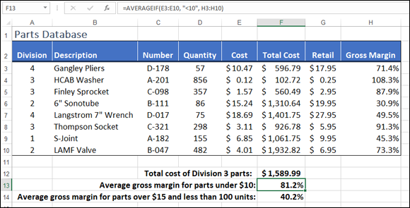
FIGURE 11-2: A parts database.

But if, instead, you want the average of the Gross Margin values, but only for those parts with a Cost value under $10, you're into AVERAGEIF territory:

=AVERAGEIF(E3:E10, "<10", H3:H10)

This function says to Excel, in effect, “look in the range E3:E10, and each time you come across a value that’s less than 10, grab the corresponding value from the range H3:H10 and include that value in the average. Best regards, AVERAGEIF.”

Calculating an average based on multiple conditions

If you want to calculate an average based on multiple criteria applied to one or more ranges, check out the AVERAGEIFS function:

=AVERAGEIFs(average_range, range1, criteria1[, range2, criteria2…])

The average_range argument is the range from which you want the average values to be taken. criteria1 gets applied to range1, criteria2 gets applied to range2, and so on. AVERAGEIFS includes in the calculation only those cells that match all the criteria.

Referring back to the parts database shown in Figure 11-2, suppose you want the average of the Gross Margin values, but only for those parts with a Quantity value (D3:D10) less than 100 and a Cost value (E3:E10) greater than $15. AVERAGEIFS is on it:

=AVERAGEIFS(H3:H10, D3:D10, "<100", E3:E10, ">15")

This formula appears in cell F14 of Figure 11-2, and you can see that the result is 40.2%.

Calculating the median

When analyzing data, you may need to find the median, which is the midpoint in a series of numbers: the point at which half the values are greater and half the values are less when you arrange the values in numerical order. What about when you have an even number of values? Great question! In that case, the median is the average of the two values that lie in the middle.

To calculate the median, you use Excel's MEDIAN function:

MEDIAN(number1[, number2, …])

You can enter up to 255 arguments, and each can be a number, cell, range, range name, or array. Excel includes zeroes in the calculation, but not blanks.

In the Product Defects worksheet shown in Figure 11-3, the median value of the Defects column (D3:D19) is given by the following formula in cell I2:

=MEDIAN(D3:D19)

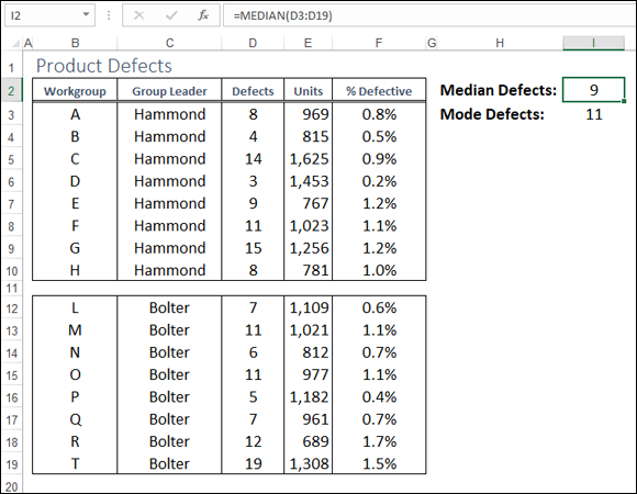
FIGURE 11-3: MEDIAN returns the median value of a set of numeric values.

Calculating the mode

The mode is the most common value in a list of values. To calculate the mode for a set of numbers, fire up Excel’s MODE function:

MODE(number1[, number2, …])

You can specify up to 255 arguments; each argument can be a number, cell, range, range name, or array. Excel includes zeroes in the calculation, but it doesn’t include blanks.

In the Product Defects worksheet, shown earlier in Figure 11-3, the mode value of the Defects column (D3:D19) is given by the following formula in cell I3:

=MODE(D3:D19)

Excel interprets the logical value TRUE as 1 and the logical value FALSE as 0, so you can use logical values as arguments when calculating the median or mode. However, if an array or a range of cells contains a logical value, MEDIAN and MODE don't include them in the calculation.

Finding the Rank

Finding how one item ranks relative to the other items in a list is often useful. For example, you might want to find out how a student’s test score ranks in relation to the other students. You can do this by sorting the list, but in some situations, sorting isn’t advisable. For example, if the original data was constantly changing, it would require constant resorting. Instead, you can use Excel’s RANK.EQ function to determine an item's rank relative to other items in a list:

RANK.EQ(number, ref[, order])

RANK.EQ takes three arguments: number is the item you want to rank; ref is the range that holds the list of items; and order is the optional sort order you want Excel to use. The default is descending, but you can use any nonzero value for ascending.

For example, Figure 11-4 shows a worksheet that contains student grades in the range B3:B48. To find out the rank of the grade in cell B3, you use the following formula:

=RANK.EQ(B3, $B$3:$B$48)

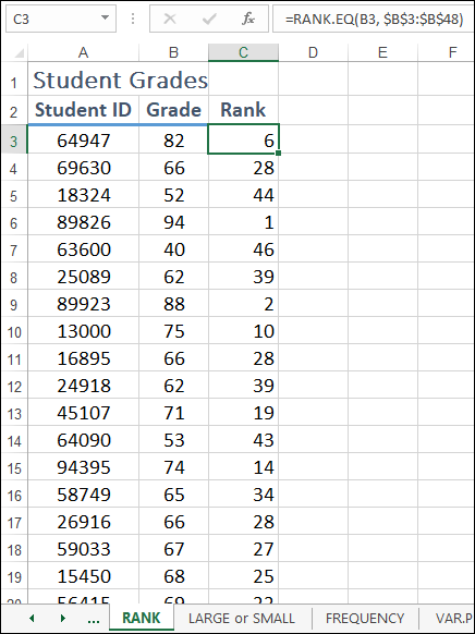
FIGURE 11-4: RANK returns the ranking of a value in a set.

As you can see in cell C3, the returned value is 6.

Note the use of absolute references for the ref argument in Figure 11-4. I used absolute references because after entering the formula in cell C3, I filled the formula down from C4 to C48. By using an absolute range reference, I ensured that the ref argument is the same for all the filled cells.

You can also use the RANK.AVG function to calculate the rank. With RANK.AVG, if two or more numbers have the same rank, Excel averages the rank. For example, in the list 100, 95, 90, 85, 85, 80, 70, the RANK.AVG function ranks the number 85 as 4.5, which is the average of 4 and 5. By contrast, RANK.EQ would give both instances of 85 the rank 4. With both RANK.EQ and RANK.AVG, if two or more numbers have the same rank, subsequent numbers are affected. In the preceding list, the number 80 ranks sixth. The RANK.AVG function takes the same three arguments as RANK.EQ:

RANK.AVG(number, ref[, order])

While you're here, I might as well mention Excel’s PERCENTRANK.INC function, which you can wield to determine the rank of a value as a percentage of all the values in your data set. PERCENTRANK.INC takes three arguments:

PERCENTRANK.INC(array, x[, significance])

Here, array is the array or range you want to use; x is the value you want to rank; and significance is the optional number of significant digits you want your results to return (the default is three). PERCENTRANK.INC gives equal values the same rank.

Excel also includes PERCENTRANK.EXC to comply with industry standards for calculating the rank of a value as a percentage of all the values in a data set:

PERCENTRANK.EXC(array, x[, significance])

As you can see, PERCENTRANK.EXC takes the same arguments as PERCENTRANK.INC, but it excludes the ranks of 0 and 100.

Determining the Nth Largest or Smallest Value

When given a list of values and an item from that list, you can use RANK.EQ (or RANK.AVG) to determine that item's rank (ascending or descending) within that list. A slightly different approach to this problem is to determine, given a list of values, what item in that list has a specified rank, such as first, third, or tenth.

You can solve this problem by sorting the list, but if the values change constantly, a better approach is to use Excel's LARGE or SMALL function, as I describe in the next two sections.

Calculating the nth highest value

Excel’s LARGE worksheet function returns the nth highest value in a list. Here’s the syntax:

LARGE(array, n)

LARGE takes two arguments: array is the array or range you want to work with, and n is the rank order of the value you seek.

For example, given a list of student grades shown in the range B3:B48 in Figure 11-5, what's the minimum mark required to crack the top 10 grades? That’s a piece of cake for the LARGE function, where the following formula (see cell D4 in Figure 11-5) returns the value 75:

=LARGE(B3:B48, 10)

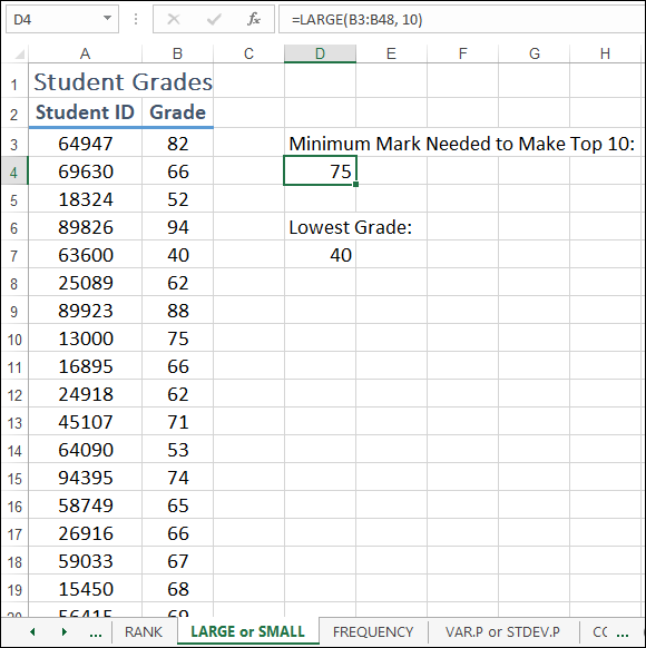
FIGURE 11-5: LARGE returns the nth largest value in a range or array.

Calculating the nth smallest value

Excel’s SMALL worksheet function returns the nth smallest value in an array or range. Here’s the syntax:

SMALL(array, n)

SMALL takes two arguments: array is the array or range you want to work with, and n is the rank order of the value you want.

For example, given the student grades shown in the range B3:B48 in Figure 11-5, what's the lowest grade? The following formula (see cell D7 in Figure 11-5) returns the value 40:

=SMALL(B3:B48, 1)

Creating a Grouped Frequency Distribution

Organizing a large amount of data into a grouped frequency distribution can help you see patterns within the data. With student test scores, for example, the first group might be scores less than or equal to 50, the second group might be 51 to 60, and so on, up to scores between 91 and 100. You can use the Excel FREQUENCY function to return the number of occurrences in each group:

FREQUENCY(data_array, bins_array)

FREQUENCY takes two arguments: data_array is the list of values you want to group; bins_array is the list of groupings (known as bins) you want to use. You enter FREQUENCY as an array formula into the same number of cells as you have groups. For example, if you have six groups, you enter the formula into six cells. Here are the steps to follow:

1. Select the cells where you want the grouped frequency distribution to appear.
2. Type =frequency(.
3. Enter or select the items you want to group.

4. Type a comma and then enter or select the list of groupings.

   When you create your frequency distribution, keep the number of groups reasonable: between five and ten is good. If you have too few or too many groups, you can lose your ability to convey information easily. Too few intervals can hide trends, and too many intervals can mask details. You should also keep your intervals simple. Intervals of 5, 10, or 20 are good because they are easy to understand. Start your interval with a value that's divisible by the interval size, which will make your frequency distribution easy to read. Finally, all intervals should have the same number of values. Again, this makes your frequency distribution easy to understand.

5. Type ).

6. Hold down Ctrl+Shift and then click the Enter button or press Ctrl+Shift+Enter.

   Excel enters the array formula and returns the number of items in each grouping. Figure 11-6 shows a FREQUENCY array formula entered into the range E3:E8.

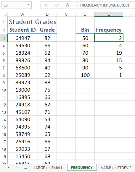
FIGURE 11-6: FREQUENCY tells you how many items in a range appear in each bin.

Calculating the Variance

Part of your analysis might involve determining how, on average, some values deviate from the mean. One method is to take the difference each number varies from the mean, square those differences, sum those squares, and then divide by the number of values. The result is called the variance, and in Excel you calculate it using VAR.S or VAR.P:

VAR.S(number1[, number2, …])
VAR.P(number1[, number2, …])

Use VAR.S if your data represents a sample of a larger population; use VAR.P if your data represents the entire population. In both cases, you can enter up to 255 arguments.

For example, in the Product Defects worksheet, shown in Figure 11-7, I calculate the variance of the Defects column (D3:D19) with the following formula (see cell H3):

=VAR.P(D3:D19)

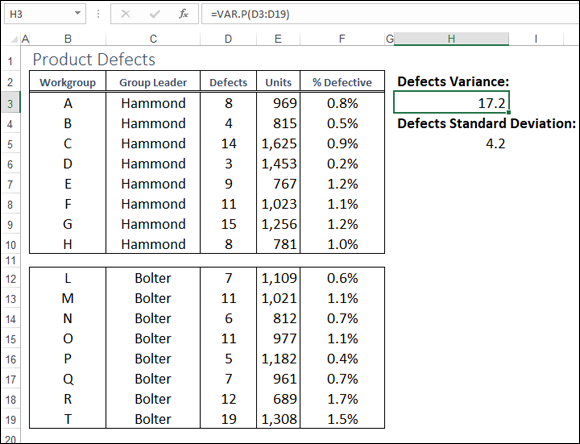
FIGURE 11-7: VAR.P returns the variance of data that represents an entire population.

Calculating the Standard Deviation

I introduce the variance in the previous section, but because the variance is a squared value, it’s difficult to interpret relative to the mean. Therefore, statisticians often calculate the standard deviation, which is the square root of the variance.

If two data sets have a similar mean, the set with a higher standard deviation has more variable data. If your data is distributed normally, about 68 percent of the data is found within one standard deviation of the mean; about 95 percent is within two standard deviations; and about 99 percent is within three standard deviations.

To calculate the standard deviation, you can use the STDEV.S or STDEV.P function.

STDEV.S(number1[, number2, …])
STDEV.P(number1[, number2, …])

Use STDEV.S if your data is a sample of a population; use STDEV.P if your data is the entire population. In both cases, you can enter up to 255 arguments.

For example, in the Product Defects worksheet shown earlier in Figure 11-7, I calculated the standard deviation of the Defects column (D3:D19) with the following formula (see cell H3):

=STDEV.P(D3:D19)

The relation of the values to each other in the data set affects the standard deviation. For example, a single outlier can distort the standard deviation, and a data set consisting of identical values gives you a standard deviation of zero.

Finding the Correlation

Correlation is a measure of the relationship between two sets of data. For example, if you have monthly figures for advertising expenses and sales, you might wonder whether higher advertising expenses lead to more sales, that is, whether the two values are related.

Keep in mind that a correlation does not prove that one thing causes another. The most you can say is that one number varies with the other.

To find a correlation in Excel, you use the CORREL function:

CORREL(array1, array2)

CORREL takes two arguments: array1 and array2, which are two lists of numbers. CORREL returns the correlation coefficient, which is a number between –1 and 1. The sign suggests whether the relationship is positive (+) or negative (–). See the following table to help interpret the result.

Correlation Coefficient	Interpretation
1	The data sets are perfectly and positively correlated. For example, a 10-percent increase in advertising produces a 10-percent increase in sales.
Between 0 and 1	The data sets are positively correlated. The higher the number is, the higher the correlation is between the data.
0	No correlation exists between the data.
Between 0 and –1	The data sets are negatively correlated. The lower the number is, the more negatively correlated the data is.
–1	The data sets have a perfect negative correlation. For example, a 10-percent increase in advertising leads to a 10-percent decrease in sales.

Figure 11-8 shows a worksheet that has advertising costs in the range C3:C14 and sales in the range D3:D14. Cell F3 calculates the correlation between these two ranges as follows:

=CORREL(C3:C14, D3:D14)

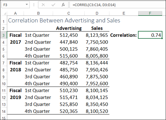
FIGURE 11-8: CORREL calculates the correlation between two sets of values.