Chapman Piloting & Seamanship

Figure 17-01 The rise and fall of ocean tidal levels cause a flow first into and then out of inland bodies of water such as bays, sounds, and the lower reaches of rivers. Because they can set a boat off its course, these tidal currents have important effects in piloting.

The Nature of Tides & Their Causes • Tidal Predictions & Calculations Currents & Their Prediction • The Effects of Currents on Piloting

An understanding of tides and currents is important to a skipper in coastal waters, as these can to some extent affect where he or she can travel or anchor safely, how long it will take to get there—or the speed that will be needed to arrive at a given time—and the heading that must be maintained to make good a given course over the bottom.

Here we should reemphasize the proper meaning and use of some terms that often are used incorrectly. TIDE is the rise and fall of the ocean level as a result of changes in the gravitational attraction between earth, moon, and sun. It is a vertical motion only. CURRENT is the horizontal motion of water from any cause. TIDAL CURRENT is the flow of water from one point to another that results from a difference in tidal heights at those points. To say “The tide certainly is running strongly today!” is not correct, for tides may be high or low, but they do not “run.” The correct expression would be “The tidal current certainly is strong today.” Remember—tide is vertical change; current is horizontal flow.

Tides originate in the open oceans and seas, but are only noticeable and significant close to shore. The effects of tides will be observed along coastal beaches, in bays and sounds, and up rivers generally as far as the first rapids, waterfall, or dam. Curiously, the rise and fall of tides may be more noticeable a hundred miles up a river than at the river’s mouth, because water piles up higher in the river’s narrower stretches. Coastal regions in which the water levels are subject to tidal action are commonly referred to as “tidewater” areas.

In addition to the basic definition of tide as given above, certain other terms used in connection with tidal action must be defined. The height of tide at any specified time is the vertical measurement between the surface of the water and the tidal datum, or reference plane, typically at what is called mean lower low water;. Do not confuse “height of tide” with “depth of water.” The latter is the total distance from the surface to the bottom. The tidal datum for an area is selected so that the heights of tide are normally positive values, but the height can at times be a small negative number when the water level falls below the datum.

HIGH WATER, or HIGH TIDE, is the highest level reached by an ascending tide; see Figure 17-02. Correspondingly, LOW WATER, or LOW TIDE, is the lowest level reached by a descending tide. The difference between high and low waters is the RANGE of the tide.

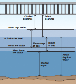
Figure 17-02 Mean lower low water is the reference level for all NOS tide levels. Bridge clearances are measured from mean high water. Tidal range is the difference between a given high water and the adjacent low water. Mean range of tide is the difference between mean low water and mean high water.

The change in tidal level does not occur at a uniform rate; starting from low water, the level builds up slowly, then at an increasing rate which in turn tapers off as high water is reached. The decrease in tidal stage from high water to low follows a corresponding pattern of a slow buildup to a maximum rate roughly midway between stages, followed by a decreasing rate. At both high and low tides, there will be periods of relatively no change in level; these are termed STAND, as in the high-water stand and the low-water stand. MEAN SEA LEVEL is the average level of the open ocean, and corresponds closely to mid-tide levels offshore; it is not used in navigation.

Tidal theory involves the interaction of gravitational and centrifugal forces—the inward attractions of the earth on one hand and the sun and the moon on the other, balanced by the outward forces resulting from the revolution of the earth in its orbit; see Figure 17-03. The gravitational and centrifugal forces are in balance as a whole—otherwise the bodies would fly apart from each other or else crash together—but they are not quite in balance at most points on the earth’s surface, and this is what causes the tides. The effects of the sun and moon will be described separately, even though, of course, they act simultaneously.

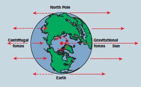
Figure 17-03 Tides result from the differences between centrifugal and gravitational forces. The forces illustrated here represent the interaction of the earth and sun; corresponding forces result from the relationship of the moon and the earth.

Although not precisely the case, the earth can be thought of as revolving around the sun, and just as a stone tied to the end of a string tends to sail off when a young boy whirls it about his head, so the earth tends to fly off into space. This effect is known as centrifugal force; it is shown at the left in Figure 17-03. (Remember that we are talking about the centrifugal force related to the sunearth system, and not that of the spinning of the earth on its own axis.)

The earth is kept from flying off into space by the gravitational attraction of the sun, shown at the right in Figure 17-03. These forces are in overall balance.

This balance of forces is not exact at all points. The sun-earth centrifugal force acts opposite to the direction toward the sun; since centrifugal force increases with the radius of rotation, it is greatest on the side of the earth that is away from the sun. Gravitational forces increase as the distance between objects decreases, therefore the gravitational force acting toward the sun is greatest on the side of the earth that is closest to the sun. Figure 17-03 shows these forces.

In theory, we can think of the earth as being a smooth sphere uniformly covered with water (no land areas). Figure 17-04 shows how the resultant forces cause the water to flow toward the areas of the earth’s surface that are both nearest and farthest from the sun; here there will be “high tides.” As this water flows, the areas from which it comes will have less water, and hence low tides. (The tides on the side of the earth nearer the sun are slightly greater than those on the far side, but the difference is not great—only about 5 percent.)

As the earth rotates on its axis once every 24 hours, the line of direction to the sun constantly changes. Thus each point of the earth’s surface will have two high and two low tides each day. As a result of the tilt of the earth’s axis, the pairs of highs, and those of the lows, will not normally be of exactly the same level.

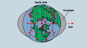
Figure 17-04 In a theoretical simplification, high tides are created on opposite sides of the earth at the same time. The gravitational attraction of the sun (or moon) pulls one way and the centrifugal force of the earth’s orbit pulls the other way.

The moon is commonly thought of as revolving about the earth; actually, the two bodies revolve around a common point on a monthly cycle. This point is located about 2,900 miles (4,667 km) from the center of the earth toward the moon (about 1,100 miles or 1,770 km deep inside the earth). Both tend to fly away from this common point (centrifugal force), but the mutual gravitational attraction acts as a counterbalance and they remain the same distance apart. However, the gravitational pull of the moon affects the waters of the earth in the same manner as the pull of the sun.

Now combine the earth-sun and the earth-moon systems. Although the mass of the moon is only a tiny fraction of that of the sun, it is much closer to the earth (about 238,860 miles or 384,400 km away). Thus its tidal forces are roughly 2¼ times greater than those of the sun (about 92,900,000 miles or 149,500,000 km away). The result is that the observed tide usually “follows the moon,” but the action is somewhat modified by the sun’s relative position. The two high and two low waters each day occur about 50 minutes later than the corresponding tides of the previous day.

In the course of any one lunar month, the three bodies line up in sun-moon-earth and sun-earthmoon relationships; see Figure 17-05. These are the times of the new and full moon, respectively. In both cases, the sun’s effect lines up with and reinforces the moon’s effect, tending to result in greater than average tidal ranges (usually about 20 percent) called SPRING TIDES; note that this name has nothing to do with the season of the year.

At other positions in Figure 17-05, when the moon is at its first and third quarters, the tidal “bulge” caused by the sun is at right angles to that caused by the moon (they are said to be “in QUADRATURE”). The two tidal effects are in conflict and partially cancel each other, resulting in smaller-than-average ranges (again about 20 percent); these are NEAP TIDES.

Note that the tidal range of any given point varies from month to month, and from year to year. The monthly variation results from the fact that the earth is not at the center of the moon’s orbit. When the moon is closest to the earth (at PERIGEE), the lunar influence is maximum and tides will have the greatest ranges. Conversely, when the moon is farthest from the earth (at APOGEE), its effect and tidal ranges are least.

In a similar manner, the yearly variations in the daily ranges of the tides are caused by the changing gravitational effects of the sun as the body’s distance from the earth becomes greater or less.

Figure 17-05 At new and full moons, the combined gravitational pull of the sun and the moon produces the largest tidal variations. These tides, which occur twice a month, are called spring tides. At the first and third quarters of the moon, the two gravitational forces partially offset each other and the net tidal effect is less; these tides are called neap tides.

The tide that we observe often seems to be at odds with the theoretical forces that govern it. Here are the main reasons for this:

• Great masses of land, the continents, irregularly shaped and irregularly placed, act to interrupt, restrict, and reflect tidal movements.

• Water, although generally appearing to flow freely, is actually a somewhat viscous substance that lags in its response to tidal forces.

• The depth to the bottom of the sea, varying widely, influences the speed of the horizontal tidal motion.

• The depths of the ocean areas and the restrictions of the continents often result in “basins” that have their own way of responding to tidal forces.

Although these reasons account for great differences between theoretical and observed tides, there nevertheless remain definite, constant relationships between the two at any particular location. By observing the tide and relating these observations to the movements of the sun, moon, and earth, these constant relationships can be determined. With this information, tides can be predicted for any future date at a given place.

A tide that each day has two high waters approximately equal in height, and two low waters also about equal, is known as a SEMIDIURNAL tide. This is the most common tide, and, in the United States, occurs along the East Coast; see Figure 17-06, left.

In a monthly cycle, the moon moves north and south of the equator; the importance of this action to tides is illustrated in Figure 17-07. Point A is under a bulge in the envelope. A half day later, at point B, it is again under the bulge but the height is not as large as A. This situation, combined with coastal characteristics, tends to give rise to a “twice daily” tide with unequal high and/or low waters in some areas. This is known as the MIXED type of tide; refer to Figure 17-06, center. The term “low water” may be modified to indicate the more pronounced of the two lows. This tidal stage is termed LOWER LOW WATER and is averaged over a complete tidal cycle of approximately 19 years to determine the MEAN LOWER LOW WATER (MLLW), which is used as the tidal datum in many areas; refer to Figure 17-02. Likewise, the more significant of the higher tides is termed HIGHER HIGHWATER.

Figure 17-06 The daily cycle of tides (a 24-hour period is shown in blue) varies widely from place to place. There are three basic types—semidiurnal (left), mixed (center), and diurnal (right).

Now consider point C in Figure 17-07. At this place, it is still under the bulge of the envelope. Point D, however, which is at the same latitude as point C, it is above the low part. Point C will reach the orientation of point D after one half day of the earth’s rotation. Hence the tidal forces tend to cause only one high and one low water each day (actually each 24 hours and 50 minutes approximately). This is the DIURNAL type, typified by Pensacola, Florida; refer to Figure 17-06, right.

Whenever the moon is farthest north (as in Figure 17-07) or south, there will be a tendency to have the diurnal or mixed type. When the moon lies over the equator, we tend to have the semidiurnal type. These are EQUATORIAL TIDES, and the tendency toward producing inequality is then at a minimum.

These theoretical considerations are modified, however, by many practical factors such as the general configuration of the coastline.

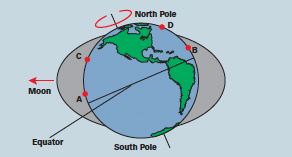
Figure 17-07 As the moon travels north and south of the earth’s equatorial plane, it causes variations in the daily cycle at any given location on earth. Similar but smaller effects result from the sun’s change in position with respect to the equator.

Peculiarities in the tide can be found almost everywhere, but none compare with those in the Bay of Fundy of eastern North America. Twice each day, the waters surge in and out of the Bay producing, at Burntcoat Head, the highest tidal range in the world, a typical rise and fall of nearly 44 feet (13.4 meters). At normal spring tides, it rises 51.5 feet (15.7 m), and on perigee springs, as much as 53 feet or 16.2 meters.

The great range is often attributed to the funnel-like shape of the bay, but this is not the main cause. Just as the water in a washbasin will slosh when you move your hand back and forth in just the right period of time, depending upon the depth of the water and the shape of the basin, so the tide will attempt to oscillate water in bays in cycles of 12 hours and 25 minutes. It would be a coincidence, indeed, if a bay were of such a shape and depth as to have a complete oscillation with a period of exactly 12 hours and 25 minutes. A bay can easily have a part of such an oscillation, however, and such is the case in the Bay of Fundy.

A further factor in the large tidal ranges in the Bay of Fundy is that they are significantly affected by the Gulf of Maine tides, which, in turn, are affected by the open ocean tides. The relationships between these tides are such as to exaggerate their ranges.

As mentioned, the heights of tides are reckoned from the specific reference plane, or datum. Although in the past, different datums were used on the Atlantic, Gulf, and Pacific Coasts of the United States, for all areas the predictions and charts of the National Ocean Service (NOS) are now based on a datum of mean lower low water.

A good knowledge of tidal action is essential for safe navigation. The skipper of a boat of any size will be faced many times with the need to know the times of high water and low water and their probable heights. He may want to cross some shoal area, passable at certain tidal stages but not at others. He may be about to anchor, and the scope to pay out will be affected by the tide’s range. He may be going to make fast to a pier or wharf in a strange harbor and needs to know about the tides to adjust his lines properly for the night.

The basic source of information on the times of high and low water and their heights above (or below) the datum are the TIDE TABLES prepared by the National Ocean Service. NOS no longer prints these tables for sale to the public, but rather provides the data to several commercial contractors who do the printing in book format annually in four volumes, one of which covers the East Coast of North and South America, and another the West Coast of these continents; refer to Chapter 15, Figure 15-38. The printed Tide Tables can usually be bought at any authorized sales agent for NOS charts or a nautical bookstore. The NOS tide data are also used by companies that prepare programs of tidal information for personal computers and other electronic devices.

For information on predictions, contact NOAA/National Ocean Services, CO-OPS, 1305 East-West Highway, Silver Spring, MD 20910-3281; phone 301-713-2815; fax 301-713-4500; or visit the NOAA website. From this URL you can access tide predictions for any station. You can download for viewing or saving the annual predictions for the station of interest in the format shown in Figures 17-08, 17-09, and 17-11, or you can select the day or days of particular interest.

Any predictions appearing in newspapers or broadcast over radio and TV stations will have been extracted from these tables. Small-craft charts may include tidal information in their margins or on the cover jacket, if one is used; see Figure 17-08.

The Tide Tables give the predicted times and heights of high and low water for each day of the year at important points known as REFERENCE STATIONS. Portland, Boston, Sandy Hook, and Key West are examples of points for which detailed information is given in the East Coast Tide Tables. Reference stations in the West Coast Tide Tables include San Diego, the Golden Gate at San Francisco, and Aberdeen, Washington.

Additional data show the difference in times and heights between these reference stations and thousands of other points termed SUBORDINATE STATIONS. From these tables, the tide at virtually any point of significance along the coasts can easily be computed. The West Coast Tide Tables, for example, contain predictions for 40 reference stations and differences for about 1,100 subordinate stations in North and South America.

Figure 17-08 Small-craft charts provide annual tidal predictions for reference stations covered by the chart. Information tabulated for marinas and other boating facilities includes data on the mean tidal range and the time difference from the applicable reference station.

All factors that can be determined in advance are taken into account in tide predictions, but remember when using them that other factors can also influence the height of tides greatly. Such influences include barometric pressure and wind. In many areas the effect of a prolonged gale from a certain quarter can offset all other factors. Tidal rivers may be affected by the volume of water flowing down from the watershed. Normal seasonal variations of flow are allowed for in the predictions, but unexpected prolonged wet or dry spells may cause significant changes to tidal height predictions. Intense rainfall upriver may change both heights and times of tides, and such effects may not appear downstream for several days.

You should therefore be careful whenever using the Tide Tables, especially since low waters can go considerably lower than the level predicted.

Figure 17-09 Each reference station is given four pages in Table 1, and each page covers three months. Tide levels are shown in feet and centimeters. The days of new and full moons are also indicated.

Table 1 of the Tide Tables gives the predicted times and heights of high and low water at the main reference stations and is self-explanatory; note that heights are given in both feet and meters or centimeters; see Figures 17-09, 17-10, and 17-11. Where no sign is given before the predicted height, the quantity is positive and is to be added to the depths as given on the chart. When the value is preceded by a minus (-) sign, the “heights” are to be subtracted from charted depths.

Figure 17-10 This Table 1 extract shows how a high or low tide may be omitted near midnight (see text); this might occur about once every two weeks.

Time is given in the four-digit system from 0001 to 2400. In many areas you must be careful regarding daylight time (DT). The Tide Tables may be published in local standard or daylight time, and a correction may be required. Tide predictions on NOAA's website are corrected for daylight time if you choose the default setting, but you can, as an option, choose standard time instead.

When there are normally two high and two low tides each date, they are roughly a little less than an hour later each succeeding day. Consequently, a high or low tide may skip a calendar day, as indicated by a blank space in the Tide Tables; see Figure 17-10. If it is a low tide that is skipped, for example, you will note that the previous corresponding low occurred late in the foregoing day, and the next one will occur early in the following day; see the sequence for late nighttime high tides on the 16th, 17th, and 18th in Figure 17-10; and refer to Figure 17-06, center.

Note also from a review of the Tide Tables that at some places there will be only one high and one low tide on some days, with the usual four tides on other days. This is not a diurnal tide situation, where a single high and low would occur every day. The condition considered here arises when the configuration of the land and the periods between successive tides are such that one tide is reflected back from the shore and alters the effect of the succeeding tide.

Sometimes the difference in the height of the two high or two low waters of a day is so increased as to cause only one low water each day. These tides are not unusual in the tropics and consequently are called TROPIC TIDES.

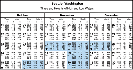
Figure 17-11 This is an extract from Table 1; it is used for working the examples of tide-level calculations.

Table 2, Tidal Differences and Other Constants, gives the information necessary to find the time and height of tide for thousands of subordinate stations by applying simple corrections to the data given for the main reference stations; see Figures 17-12 and 17-13. The name of the applicable reference stations appears at the head of the particular section in which the subordinate station is listed. After the subordinate station number and name, the following information is given in the columns of Table 2:

2. Differences in time and height of high (and low) waters at the subordinate station and its designated reference station.

Figure 17-12 This is an extract from Table 2 to be used in working the text examples. Note that the differences are to be applied to the Seattle reference station as indicated in the fourth column. Asterisks (*) indicate ratios. The height at the reference station is multiplied by this figure; see text.

As mentioned, note that the existence of a “minus tide” means that the actual depths of water will be less than the figures on the chart.

To determine the time of high or low water at any station in Table 2, use the column marked “Differences, Time.” This gives the hours and minutes to be added to (+) or subtracted from (-) the time of the respective high or low water at the reference station shown in boldface type above the listing of the subordinate station. Be careful in making calculations near midnight. Applying the time difference may cause you to cross the line from one day to another. Simply add or subtract 24 hours as necessary.

The height of the tide at a station in Table 2 is determined by applying the HEIGHT DIFFERENCE, or in some cases the RATIO. A plus sign (+) indicates that the difference increases the height given for the designated reference station; a minus sign (-) indicates that it decreases the Table 1 value. Differences are not given in metric values; if needed, conversions from feet can be made using Table 7 in the Tide Tables; see also Appendix D.

Where height differences would give unsatisfactory predictions, ratios may be substituted for heights. Ratios are identified by an asterisk, and are given as a decimal fraction by which the height at the reference station is to be multiplied to determine the height at the subordinate station.

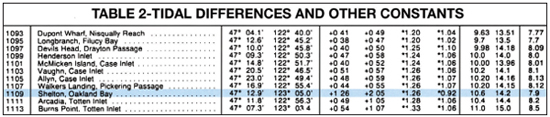
Figure 17-13 Another extract from Table 2 used in working the tide-level examples in the text. Seattle is again the reference station.

Note that when you access tide predictions at NOAA's website for a particular day or few days of interest at a subordinate station, the Table 2 corrections are applied for you, and the corrected data are ready for use. Annual predictions for a subordinate station are given in the traditional uncorrected format, however, and Table 2 corrections must be applied.

In the Table 2 columns headed “Ranges,” the MEAN RANGE is the difference in height between mean high water (MHW) and mean low water (MLW). This figure is useful in many areas where it may be added to mean low water to get mean high water, the datum commonly used for measuring vertical heights above water for bridge and other vertical clearances. The SPRING RANGE is the average semidiurnal range occurring twice monthly when the moon is new or full. It is larger than the mean range where the type of tide is either semidiurnal or mixed, and is of no practical significance where the tide is of the diurnal type. Where this is the situation, the tables give the DIURNAL RANGE, which is the difference in height between mean higher high water and mean lower low water.

Special conditions at certain subordinate stations are covered by endnotes following Table 2. The format may vary slightly with different commercial publishers.

Table 3, Height of Tide at Any Time, is provided in order that detailed calculations can be made for the height of the tide at any desired moment between the times of high and low waters; see Figure 17-14. It is equally usable for either the reference stations in Table 1 or the subordinate stations of Table 2. Note that Table 3 is not a complete set of variation from one low to one high. Since the rise and fall are assumed to be symmetrical, only a half table need be printed. Calculations are made from a high or low water, whichever is nearer to the specified time. In using Table 3, the nearest tabular values are used; interpolation is not necessary.

If the degree of precision of Table 3 is not required (it seldom is in practical piloting situations), a much simpler and quicker estimation can be made by using the following “one-twothree” rule of thumb. The tide may be assumed to rise or fall ¹/₁₂ of the full range during the first and sixth hours after high and low water stands, ²/₁₂ during the second and fifth hours, and ³/₁₂ during the third and fourth hours. The results obtained by this rule will suffice for essentially all situations and locations, but should be compared with Table 3 calculations as a check when entering new areas.

Other Tables. The Tide Tables also include four other minor tables that, although not directly related to tidal calculations, are often useful. Table 4 provides sunrise and sunset data at five-day intervals for various latitudes. Table 5 lists corrections to convert the local mean times of Table 4 to standard zone time. Table 6 tabulates times of moonrise and moonset for certain selected locations. Table 7 allows direct conversion of feet to meters. The inside back cover of the publication lists other useful data such as the phases of the moon, solar equinoxes, and solstices.

Table 1 through Table 6 are each preceded by informative material that should be read carefully prior to use of the table concerned.

Figure 17-14 Table 3 is used to determine the height of the tide at intermediate times between high and low water. To use this table, you must know three things—how long in hours and minutes between the high and low on either side of the time in which you are interested; the time in hours and minutes from that time to the nearer of the adjacent high and low; and the size of the rise or fall to the nearest half foot. The answer produced from that data and Table 3 will give you a correction value to be applied to that high or low prediction.

The tide’s rise and fall changes the vertical clearance under fixed structures such as bridges or overhead power cables. These clearances are stated on charts and in Coast Pilots as heights measured from a datum that is not the same plane as used for depths and tidal predictions. The datum for heights is normally mean high water, the average of all high water levels. The use of this datum ensures that clearances and heights are normally (though not always) greater than charted or Coast Pilot values.

It will thus be necessary to determine the height of MHW above the tidal datum. Since the tidal datum is mean lower low water, the plane of mean high water is above MLLW by an amount equal to the sum of the “mean tide level” plus one-half of the “mean range”; both of these values are listed in Table 2 of the Tide Tables for all stations; also refer to Figure 17-02.

If the tide level at any given moment is below MHW, the vertical clearance under a bridge or other fixed structure is then greater than the figures shown on the chart; but if the tide height is above the level of MHW, the clearance is less. You should calculate the vertical clearance in advance if you anticipate a tight situation, but also observe the clearance gauges usually found at bridges. Clearances will normally be greater than the charted MHW values, but will occasionally be less.

The instructions in the Tide Tables should be fully adequate for solving any problem. However, Tide-Level Examples 1 through 6 are worked here for various situations as guides to the use of various individual tables. Comments and cautions relating to the solution of practical problems involving the Tide Tables will also be given. The extracts from the Tide Tables that are necessary to work the Tide-Level Examples are given in Figures 17-11 through 17-14.

TIDE-LEVEL EXAMPLE 1

Determining the time and height of a high or low tide at a Reference Station.

Problem:What is the predicted time and height of the evening low tide at Seattle, Washington, on Monday 13 December?

Solution: Refer to the Table 1, excerpt in Figure 17-11, taken from theTideTables. Note that the entry for 13 December shows that the evening low water is predicted to occur at 2246 Pacific Standard Time (PST) and that the height will be -2.9 feet, or 2.9 feet below the tidal datum of MLLW. Actual depths will then be lower than the charted depths.

On the same date, morning low tide is 7.3 feet above the tidal datum of MLLW.

Note that on Wednesday 15 December, there is no evening low because the progression of the tides on a 24 hour and 50 minute cycle has moved the evening low tide past midnight into the next day. As a result, the table shows only three entries for Wednesday 15 December rather than the usual four.

CURRENT is the horizontal motion of water. It may result from any one of several factors, or from a combination of two or more. Although certain of these causes are more important to a boater than others are, he or she should have a general understanding of all.

The major causes of current flow are gravitational action, the flow of air (wind) across the surface of bodies of water, and geophysical differences such as variations in heat and salt. Water naturally flows “downhill” as in rivers or from higher tidal levels to lower ones. Persistent winds across large bodies of water cause a surface flow. Currents over large areas in oceans may be either seasonal or semipermanent.

Boaters in coastal areas will be affected most by TIDAL CURRENTS. The rise and fall of tidal levels is a result of the flow of water to and from a given locality. Such flow of water results in tidal current effects.

TIDE-LEVEL EXAMPLE 2

Determining the time and height of a high or low tide at a Subordinate Station.

Problem:What is the predicted time and height of the morning low water atYokeko Point, Deception Pass, on Saturday 13 November?

Solution:The Index to Table 2 in the TideTables showsYokeko Point as Subordinate Station number 1147. Locate Yokeko Point in Table 2 and note the time and height differences for low waters; be sure to use the correct columns.

Apply the difference to the time and height of low tide at the Reference Station as follows:


Time		Height
09 53	at Seattle	5.9
+0:38	difference	-0.2
10 31	at Yokeko Point	5.7

Thus atYokeko Point, on 13 November, the predicted morning low will occur at 1031 PST with a height of 5.7 feet above tidal datum.

Note: If the example had been November 30, the morning low water at Seattle for that date is at 1140. Adding the time difference of 0h 38m would have resulted in a time prediction at Yokeko Point of 1218, which is not a morning tide. In such cases, use the reference station low water that occurs before midnight the preceding day.

The normal type of tidal current, in bays and rivers, is called the REVERSING current that flows alternately in one direction and then in the opposite. Off shore, tidal currents may be of the ROTARY type, flowing with little change in strength, but while slowly and steadily changing direction.

A special form of a tidal current is known as the HYDRAULIC type, such as flows in a waterway connecting two bodies of water. Differences in the time and height of the high and low waters of the two bays, sounds, or other tidal waters cause a flow from one to the other and back again. A typical example of hydraulic current is the flow through the Cape Cod Canal between Massachusetts Bay and Buzzards Bay.

Remember to use the terms correctly—tide is the vertical rise and fall of water levels; current is the horizontal flow of water.

TIDE-LEVEL EXAMPLE 3

Determining the level of the tide at a reference station at a given time between high and low waters.

Problem:What is the predicted height of the tide at Seattle at 1700 on Sunday 28 November?

Solution: From Table 1, note that the given time of 1700 falls between a high tide at 1505 and a low tide at 2223.We compute the duration of fall and range as follows:

Time	Height
15 05	10.5
22 23	-1.1
7:18 duration of fall	11.6 feet range

The desired time is nearer to the time of high water, so calculations will be made using this starting point.

1700	desired time
1505	time of nearest high water
1:55	difference

The given time is 1 h 55m after the nearest high water. Turn to Table 3, which is used to the nearest tabulated value; do not interpolate. Enter the upper part of the table on the line for duration of rise or fall of 7 h 20m (nearest value to 7h 18m) and read across to the entry nearest 1h 55m—in this case 1h 57m in the eighth column from the left. Follow down this column into the lower part of Table 3 to the line for range of tide of 11.5 feet (nearest value to 11.6). At the intersection of this line and column is found the correction to the height of the tide: 1.9 feet.

Since, as we have noted, the tide is falling, and we are calculating from high water, the correction is subtracted from the height of high water:

10.5 – 1.9 = 8.6 feet.

Thus, the predicted height of the tide at Seattle at 1700 PST on Sunday 28 November is 8.6 feet above the tidal datum.

Make sure that calculations are made for the right pair of high and low tides—and that the calculations are made to the nearest high or low water. Also, be careful to apply the final correction to the nearest high or low water as used in the computation. Do not apply it to the range. Apply it in the right direction: down from a high or up from a low.

TIDE-LEVEL EXAMPLE 4

Determining the predicted height of tide at a Subordinate Station at a given time.

Problem:What is the predicted height of the tide at Shelton, Oakland Bay, Puget Sound, at 2000 on Saturday 30 October?

Solution: First, use the steps fromTide-Level Example 2—find Shelton in the index, locate its number on Table 2 and note the time and height differences. Now, the times of the high and low waters on either side of the stated time must be calculated for the subordinate station using Tables 1 and 2. This is done as follows:


High-water time	Height
15 51 at Seattle	10.4 feet
+1:26 difference	.26 ratio
17 17 at Shelton	13.1 feet

Low-water time	Height
22 48 at Seattle	-0.4
+2:05 difference	0.92 ratio
00 53 at Shelton	-0.37 (-0.4)

Next we calculate the time difference and range:

Time	Range
00 53 low water	-0.4
17 17 high water	13.1
7:36 time difference	13.5 feet range

The time from the nearest high or low is calculated:

17 17 high water at Shelton

20 00 desired time

2:43 time from nearest high

With the data from the above calculations, enter Table 3 for a duration of rise or fall of 7h 40m (nearest to 7h 36m), a time from nearest high or low of 2 h 49m (nearest to 2h 43m), and a range of 13.5 feet.

From these data, we find a correction to height of tide of 4.0 feet. We know that the tide is falling and therefore the height at 2000 will be less than the height at the closest high water at 1717. Therefore, the correction is to be subtracted from the Shelton high water height: 13.1 – 4.0 = 9.1 feet. The height of the tide at Shelton, Oakland Bay, Puget Sound, at 2000 on Saturday 30 October is predicted to be 9.1 feet above datum.

Note: If the times for 30 October in Table 1 are in PST, you’ll have to add an hour for daylight savings time. Also, you must be sure to use the high and low tides occurring at the Subordinate Station on either side of the given time. In some instances, you may find that when you have corrected the times for the subordinate station, the desired time no longer falls between the corrected times of high and low tides. In this case, select another high or low tide so that the pair used at the subordinate station will bracket the given time.

TIDE-LEVEL EXAMPLE 5

Determining the time of the tide reaching a given height at a Reference Station.

Problem: At what time on the morning ofTuesday 30 November will the height of the rising tide at Seattle reach 3 feet?

Solution:This is essentially Tide-Level Example 3 in reverse. First determine the range and duration of the rise (or fall) as follows:

Time	Height
22 56 (29th low water)	-1.4 feet
06 25 high water	12.0 feet
7:29 duration/range	13.4 feet range

It is noted that the desired difference in height of tide is from the low water –1.4 –3 = -4.4 or 4.4 feet.

Enter the lower part of Table 3 on the line for a range of 13.5 feet (nearest to actual 13.4 feet) and find the column in which the correction nearest 4.4 is tabulated: in this case, the nearest value (4.7) is found on the 12th column to the right.

Proceed up this column to the line in the upper part of the table for a duration of 7h 20m (nearest to the actual 7h 29m).The time from the nearest high or low found on this line is 2h 56m. Since our desired level is nearest to low water than high, this time difference is added to the time of low water: 2256 + 2:56 = 0152.

Thus the desired tidal height of 3 feet above datum is predicted to occur at 0152 PST on 30 November.

Note: a similar calculation can be made for a subordinate station by first determining the applicable high and low water times and heights at that station.

TIDE-LEVEL EXAMPLE 6

Determination of predicted vertical clearance.

Problem:What will be the predicted vertical clearance under the fixed bridge across the canal near Ala Spit, Whidbey Island, at the time of morning high tide on 13 December?

Solution: Chart 18445 states the clearance to be 35 feet. The datum for heights is MHW.

From Tables 1 and 2, we determine the predicted height of the tide at the specified time as follows:

At Seattle	12.7 feet
Ratio	0.92
At Ala Spit	11.68 (11.7)

From Table 2 we calculate the height of mean high water for Ala Spit.


Mean tide level	6.1 feet
½ mean range	3.5
Mean high water	9.6 feet above tidal datum

The difference between predicted high water at the specified time and mean high water is 11.7 –9.6 = 2.1This is above MHW and the bridge clearance is reduced; 35 – 2.1 = 33 feet, to the nearest whole foot.

On the morning of 13 December, the clearance at high tide under the fixed bridge across the canal near Ala Spit, Whidbey Island, is predicted to be 33 feet.This is less than the clearance printed on the chart.

Boaters on rivers above the head of tidal action must take into account RIVER CURRENTS. (Where tidal influences are felt, river currents are merged into tidal currents and are not considered separately.) River currents vary considerably with the width and depth of the stream, the season, and recent rainfall; refer to Chapter 22 for details. When rivers reach tidal areas, the currents there will be a combination of river flow and tidal level changes.

Offshore piloting will frequently require knowledge and consideration of OCEAN CURRENTS. These currents result from relatively constant winds such as the trade winds and prevailing westerlies. The rotation of the earth and variations in water density and salinity are also factors in the patterns of ocean currents.

The ocean currents of greatest interest to American boaters are the Gulf Stream and the California Current; see Figure 17-15. The Gulf Stream is a northerly and easterly flow of warm water along the Atlantic Coast of the United States. It is quite close to shore along the southern part of Florida, but moves progressively farther to sea as it flows northward, where it both broadens and slows.

The California Current flows generally southward and a bit eastward along the Pacific Coast of Canada and the United States, turning sharply westward of Baja California (Mexico). It is a flow of colder water and, in general, is slower and less sharply defined than the Gulf Stream, and exhibits some variation with season.

In addition to the consistent ocean currents caused by sustained wind patterns, temporary conditions may create local WIND-DRIVEN CURRENTS. Wind blowing across the sea causes the surface water to move. The extent of this effect varies, but generally a steady wind for 12 hours or longer will result in a discernible current.

For a rough rule of thumb, the strength of a wind-driven current can be taken as 2 percent of the wind’s velocity. The direction of the current will not be the same as that of the wind, if the flow is north or south, making it subject to deflection by the Coriolis force (to the right in the Northern Hemisphere) created by the earth’s rotation. The magnitude of the deflection is greatest at high latitudes and also depends on the depth of the water. Currents that set directly east or west are not affected by the Coriolis force.

Figure 17-15 Shown here are the major ocean surface currents of the world. The Gulf Stream off the East Coast of the United States and Canada and the California Current off the West Coast are those of most interest to North American boaters. Other currents exist at lower depths, as well as downwelling and upwelling.

Currents have both strength and direction. The proper terms should be used in describing each of these characteristics.

The SET of a current is the direction toward which it is flowing. A current that flows from north to south is termed a southerly current and has a set of 180 degrees. (Note the difference here from the manner in which wind direction is described—it is exactly the opposite: a wind from north to south is called a northerly wind with a direction described as 000 degrees.)

The DRIFT of a current is its speed, normally in knots, except for river currents, which are in mph (1 knot = 1.15 mph = 1.85 km/hr). Current drift is stated to the nearest tenth of a knot.

The term velocity is rarely used in connection with current, but if it is, it requires a statement of both strength and direction.

A tidal current is said to FLOOD when it flows in from the sea and results in higher tidal stages. Conversely, a tidal current EBBS when the flow is seaward and water levels fall.

As these currents reverse, there are brief periods of no discernible flow, called SLACK or SLACK WATER. The time of occurrence of slack is not the same as the time of STAND, when vertical rise or fall of the tide has stopped. Tidal currents do not automatically slack and reverse direction when tide levels stand at high or low water. High water at a given point simply means that the level there will not get any higher. Further up the bay or river, the tide will not have reached its maximum height, and water must therefore continue to flow in so that it can continue to rise. The current can still be flooding after stand has been passed at a given point and the level has started to fall.

For example, consider the tides and currents on Chesapeake Bay. High tide occurs at Baltimore some seven hours after it does at Smith Point, roughly halfway up the 140 miles from Cape Henry at the Bay’s entrance to Baltimore. On a certain day, high water occurs at 1126 at Smith Point, but slack water does not occur until 1304. The flooding current has thus continued for 1h 38m after high water was reached.

Corresponding time intervals occur in the case of low water stand and the slack between ebb and flood currents.

In many places, the time lag between a low or high water stand and slack water is not a matter of minutes but of hours. At the Narrows in New York Harbor, flood current continues for about two hours after high water is reached and the tide begins to fall, and continues to ebb for roughly two and a half hours after low-water stand. After slack, the current increases until mid-flood or mid-ebb, and then gradually decreases. Where ebb and flood last for about six hours—as along the Atlantic seaboard—current will be strongest about three hours after slack. Thus, the skipper who figures his passage out through the Narrows from the time of high water, rather than slack, will start about two and a half hours too soon and will run into an opposing current at nearly its maximum strength.

A current of any type can have a significant effect on the travel of a boat with respect to the bottom. Speed can be increased or decreased; the course made good can be markedly different from that steered. For safe and efficient navigation, a boater must know how to determine and apply current effects.

A current directly in line with a boat’s motion through the water will have a maximum effect on the speed made good, but no off-course influence. The effect can be of significance when figuring your ETA at your destination. It can even affect the safety of your boat and its crew if you have figured your fuel too closely and have run into a bow-on current.

A current that is nearly at a right angle to your course through the water will have a maximum effect on the course made good and a minor effect on the distance that you must travel to reach your destination.

Knowledge of current set and drift can assist your cruising. Select departure times to take advantage of favorable currents, or at least to minimize adverse effects. A 12-knot boat speed and a 2-knot current, reasonably typical situations, can combine to result in either a 10-knot or a 14-knot speed made good—the 40 percent gain from a favorable current over an opposing one is significant in terms of both time and fuel. For slower craft the gains are even greater: 50 percent for a 10-knot boat, 67 percent for an 8-knot craft, and 100 percent for one making only 6 knots.

Even lesser currents have significance. A ½-knot current would hinder a swimmer and make rowing a boat noticeably more difficult. A 1-knot current can significantly affect a sailboat in light breezes.

In many boating areas, there are locations where current conditions can be critical. Numerous ocean inlets are difficult or dangerous in certain combinations of current and onshore surf. In general, difficult surf conditions will be made more hazardous by an outward-flowing (ebbing) current. The topic of inlet seamanship is covered in more detail in Chapter 10. In many narrow bodies of water, the maximum current velocity is so high that passage is impossible for boats of limited power, and substantially slowed for boats of greater engine power; see Figure 17-16. Such narrow passages are particularly characteristic of Pacific Northwest boating areas, but do occur elsewhere. Currents in New York City’s East River reach 4.6 knots, and they are more than 5 knots at the Golden Gate of San Francisco. Velocities of 3.5 to 4 knots are common in much-traveled passages like Woods Hole, Massachusetts, and Plum Gut at the eastern end of Long Island Sound.

Figure 17-16 In some passages, tidal currents are so strong that all but the fastest boats must avoid running against the strongest flood and ebb. Skippers of less powerful craft must plan for passage at slack water or with a favorable current—in the right direction, a strong current can double the over-the-bottom speed of a displacement boat. And all skippers can gain to some degree from transiting when the current aids their passage.

Without experience or official information, local current prediction is always risky. For example, east of Badgers Island in Portsmouth (NH) Harbor, the maximum ebb current is predicted at less than a half knot. Yet just southwest of the same island, the tabular maximum is 3.7 knots.

One rule is fairly safe for most locations—the ebb is stronger and lasts longer than the flood. Eighty percent of all reference stations on the Atlantic, Gulf, and Pacific coasts of the U.S. report stronger currents in the ebb. This is normal because river flow adds to the ebb but hinders the flood.

On the Atlantic Coast, expect to find two approximately equal flood currents and two similar ebb currents in a cycle of about 24 hours and 50 minutes. On the Pacific Coast, however, the two floods and the two ebbs differ markedly. On the Gulf Coast, there may be just one flood and one ebb in 25 hours. In each case these patterns are, of course, generally similar to tidal action in their respective areas.

Don’t try to predict current velocity from the time that it takes a high tide to reach a given point from the sea’s entrance. Dividing the distance from Cape Henry to Baltimore by the time that it takes high water to work its way up Chesapeake Bay gives a speed of 13 knots. True maximum flood current strength is only about one knot.

Another important fact is that tidal currents at different places cannot be forecast from their tidal ranges. You would expect strong currents at Eastport, Maine, where the difference between successive high and low waters reaches as much as 20 feet. And you would be right; there are 3-knot currents there. But Galveston, Texas, with only a 2-foot range of tides, has currents up to more than 2 knots. So has Miami, with a 3-foot range, and Charleston, South Carolina, with a 6-foot range—these are stronger currents than Boston, where the range is often more than 10 feet, and as strong as at Anchorage, Alaska, where it’s as much as 35 feet from some highs to the next low.

A good forecasting rule for all oceans: expect strong tidal currents where two bays meet. The reason: tidal ranges and high water times in the two bodies of water are likely to be different.

For the coasting skipper, here is another tidal current fact that may be useful near the beach: flood and ebb don’t usually set to and from shore, but rather parallel with it. This is as true off New Jersey and Florida as it is off California and Oregon. A few miles offshore, however, and in some very large bays, the current behaves quite differently—for example, the rotary current mentioned previously in this chapter.

At any given place, current strength varies with the phases of the moon and its distance from the earth. It will be strongest when tidal ranges are greatest—near new and full moon—and weakest when tidal ranges are least: near first and last quarters. Current speed may vary as much as 40 percent above and below its average value.

The consistent relationship of tidal currents to tides in any given place means that once that relationship is empirically determined, future tidal currents can be predicted based on future tides. NOS provides data for two volumes of predictions annually; one covers the Atlantic Coast of North America and the other the Pacific Coast of North America and Asia. These books are printed and sold commercially in the same manner as the Tide Tables, and NOS also makes the data available to boaters at http://tidesandcurrents.noaa.gov.

These Tidal Current Tables include predictions of tidal currents in bays, sounds, and rivers, plus ocean currents such as the Gulf Stream. General information on wind-driven currents is also included, although these, of course, cannot be predicted a year or more ahead. Your own past experience and local knowledge are the best sources of information about how storm winds affect local waters. The two printed volumes of the Tidal Current Tables are available at most sales agents for charts and nautical publications.

The format and layout of the Tidal Current Tables is much the same as for the Tide Tables discussed earlier in this chapter. A system of reference stations, plus constants and differences for subordinate stations, is used to calculate the predictions for many points.

Table 1. There are 22 reference stations in the Atlantic Coast volume and 36 for the Pacific Coast; the Gulf of Mexico is included in the Atlantic Coast volume. For each station, there are tabulated predicted times and strengths of maximum flood and ebb currents, plus the times of slack water. The direction of the flood and ebb currents is also listed; see Figure 17-17.

Table 2. Time differences and velocity ratios are listed for hundreds of subordinate stations; see Figure 17-18. Following the station number and descriptive location, there is depth at which the reading was taken and then the latitude and longitude to the nearest minute. Time differences are given for maximum flood and ebb, and for minimum current (usually slack) before flood and before ebb. Speed ratios are tabulated for maximum current in both directions (given in degrees, true, for direction toward which current flows). Also listed are average speeds and directions, including speed at slack as currents do not always decrease fully to zero velocity. A few stations will have only the entry “Current weak and variable”; this information, even though negative in nature, is useful in planning a cruise. A number of endnotes are used to explain special conditions at various stations; these are found at the end of Table 2.

Note that when you access tidal current predictions at http://tidesandcurrents.noaa.gov for a particular subordinate station, the Table 2 corrections are applied for you, and the corrected data are ready for use.

Table 3. This ratio table is in two separate parts; one is for normal reversing currents (as in Figure 17-19) and the other (not shown) is for hydraulic currents at specified locations, and provides a convenient means for determining the current’s strength at times intermediate between slack and maximum velocity. Use the nearest tabulated values (as shown) without interpolation.

Table 4. Although slack water is only a momentary event, there is a period of time on either side of slack during which the current is so weak as to be negligible for practical piloting purposes. This period, naturally, varies with the maximum strength of the current, being longer for weak currents. Two subtables predict the duration of currents from 0.1 to 0.5 knots by tenths for normal reversing currents and for the hydraulic currents found at certain specified locations; see Figure 17-20.

Table 5. For the Atlantic Coast only, information is given on rotary tidal currents at various offshore points of navigational interest. These points are described in terms of general location and specific geographic coordinates. Predictions of velocity and direction are referred to times after maximum flood at designated reference stations.

The inside back cover of the Tidal Current Tables has the same astronomical data as is found in the Tide Tables;.

Figure 17-17 This is an extract from Table 1 of the Tidal Current Tables; it will be used in the Tidal Current Examples that appear later in this chapter. The times in this table are EDT for dates on which daylight savings time is in use.

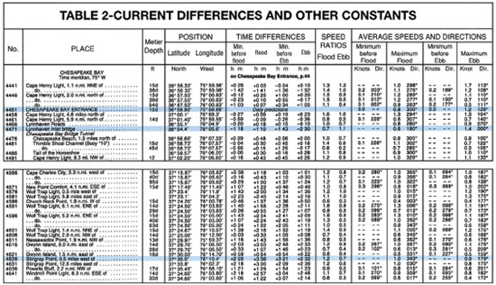
Figure 17-18 The tidal current examples in the text use this extract from Table 2 for time and speed differences to be applied to the reference station.

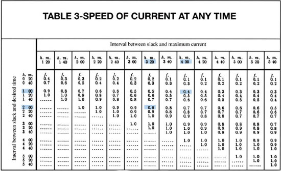
Figure 17-19 Table 3 of the Tidal Current Tables is used to determine the speed of the current at intermediate times between slack and maximum flow. It is in two parts; Table A, shown here, is used for all locations except for a few unique places that are covered in Table B (not shown).

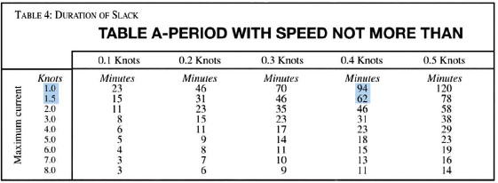
Figure 17-20 Slack is a period during which the current slows down and reverses. The length of slack is a question of how slow is slow enough. Table 4, Duration of Slack, is in two parts: Part A, shown here, is applicable in all locations except for a few that are covered in Part B (not shown). This table permits the calculation of the predicted duration of a flow that is less than, or equal to, a desired value.

Figure 17-21 A tidal current diagram, such as this one for Chesapeake Bay, helps choose the time for a passage up or down the bay at a particular speed. See the text, Tidal Current Example 6, for how it is used.

For a number of major tidal waterways of the United States, Tidal Current Tables give CURRENT DIAGRAM—graphic means for selecting a favorable time for traveling in either direction along these routes; see Figure 17-21.

Depending on publisher and format, Tidal Current Tables may list all predictions in local standard time. Be sure to make an appropriate conversion to daylight time if this is needed. Subtract an hour from your watch time before using the tables, and add an hour to the results of your calculations. (Some commercial publishers make the conversion to daylight time, and the NOS tables, when accessed online at http://tidesandcurrents.noaa.gov, can be formatted by the user to conform to daylight time or to read consistently in standard time. Check carefully the tables that you use.)

Cautions: As with tidal predictions, the data in the Tidal Current Tables may often be upset by sustained abnormal local weather conditions such as wind or rainfall. Use the current predictions with caution during and immediately after such weather phenomena.

Note also that tidal current predictions are generally for a spot location only; the set and drift may be quite different only a mile or less away. This is at variance from predictions of high and low tides, which can usually be used over fairly wide areas around the reference station.

The Tidal Current Tables contain all information needed for determining such predicted conditions as the time of maximum current and its strength, the time of slack water, and the duration of slack (actually, the duration of the very weak current conditions). Tidal current examples and solutions for typical problems follow, with comments and cautions. The extracts from the Tidal Current Tables that are necessary to work Tidal Current Examples 1 through 6 are given in Figures 17-17 through 17-21.

TIDAL CURRENT EXAMPLE 1

Determining the predicted time and strength of maximum current, and the time of slack, at a Reference Station.

Problem:What is the predicted time and strength of the maximum ebb current at Chesapeake Bay Entrance during the afternoon of 16 October?

Solution: As Chesapeake Bay Entrance is a Reference Station, the answer is available by direct inspection ofTable 1.

The table shown in Figure 17-17 is a typical page from the Tidal Current Tables. We can see that the maximum ebb current on the specified afternoon is 1.9 knots and that it occurs at 1454 EDT. An entry at the top of the page tells us that ebbs at this station have a set of 129 degrees true.

Problem:What is the predicted time of the first slack before flood at this station on 21 October?

Solution: Table 1 does not directly identify the slacks as being “slack before ebb” or “slack before flood”; this must be determined by comparing the slack time with the nature of the next maximum current that occurs.

From the table, we can see that the earliest slack that will be followed by a flooding current at Chesapeake Bay Entrance on 21 October is predicted to occur at 1000 EDT.

Notes

1. NOS formerly used local standard time but now adjusts for daylight saving time when appropriate. You may still encounter tables that are referenced strictly to standard time, however; if you do, you’ll have to add one hour to tabulated times in months when daylight saving time is in effect.

2.The direction of the current for a reference station is found at the top of the page in Table 1. It is also given in Table 2, which lists further information such as the geographic coordinates of the station.

3.The normal day at Chesapeake Bay Entrance, where the tide is of the semidiurnal type, will have four slacks and four maximums.The tidal cycle of 24h and 50m will result in the occasional omission of a slack or maximum. You can see that a slack occurs very late on 20 October; the flood that follows it occurs on the following date.

TIDAL CURRENT EXAMPLE 2

Determining the time and strength of maximum current, and the time of slack, at a subordinate station.

Problem: What is the predicted time and strength of the morning maximum flood current at Lynnhaven Inlet bridge on 16 December?

Solution:Table 2 (refer to Figure 17-18) gives time differences and velocity ratios to be applied to the predictions at the appropriate reference station. There is an index to Table 2 at the back of the Tidal CurrentTables if it is needed to locate the given subordinate station.

For Lynnhaven Inlet bridge, the time difference and speed ratio are applied as follows:

Time		Velocity
09 50	Chesapeake Bay Entrance	1.2
-1:10	Lynnhaven factor	0.7
08 40	morning flood at Lynnhaven	0.8

The set (direction) of the current is also noted from the appropriate column of Table 2; in this case, it is 180° true.Thus the predictions are for a maximum current of 0.8 knot setting 180° true at Lynnhaven Inlet bridge at 0840 on 16 December.

Problem: What is the predicted time of the first afternoon slack water at Lynnhaven Inlet bridge on 17 October?

Solution:Table 1 shows the first afternoon slack for this date (1218) as a slack before ebb begins, but the time difference of –1.18 (from Table 2) makes it a morning slack at the Subordinate Station. So the next slack, which is before flood at 1858, must be used.


18 58	Chesapeake Bay Entrance
-1:18	difference for subordinate station
17 40	at Lynnhaven Inlet bridge

Notes

1. Observe that Table 2 shows separate time differences for the four events of a tidal current cycle; always carefully check the column headings and select the proper time difference. Note also that the speed ratios for maximum flood and ebb currents are normally different.

2.The direction of the current at a subordinate station nearly always differs from that of a reference station; it must be taken from Table 2. No statement of current is complete without giving direction as well as strength.

3. If you access the Lynnhaven Inlet bridge station at http://tidesandcurrents.noaa.gov, the time and velocity differences from the Chesapeake Bay Entrance station will be applied for you.

TIDAL CURRENT EXAMPLE 3

Determining the strength and set of a current, at an intermediate time at a reference station.

Problem: What is the predicted strength and set of the current at Chesapeake Bay Entrance at 1620 on 1 October?

Solution: The times of slack and maximum current (ebb or flood) that bracket the desired time are found from Table 1. The interval between these times is determined, as is the interval between the desired time and slack.


18 11	time of nearest slack
14 56	time of maximum ebb current
3:15	interval, slack—maximum current

18 11	time of nearest slack
16 20	desired time
1:51	interval, slack—desired time

Once you have established these time intervals, Table 3A (see Figure 17-19) is used to determine the ratio of the strength of the current at the desired time to its maximum strength. The nearest tabulated values are used, with no interpolation. In this example, the ratio at the intersection of the line for 2h 00m (closest to 1h 51m) and the column for 3 h 20m (closest to 3h 15m) is found to be 0.8. Multiply the maximum current by this decimal fraction, 1.2 x 0.8 = 0.96 (which is used as 1.0).

From the times used, we note that the current is ebbing. From the top of Table 1, we determine that the direction is 129° true. So on 1 October, at 1620, the current at Chesapeake Bay Entrance will be 1.0 knots setting 129° true.

Notes

1. Except as specially indicated, use Table 3A, the upper portion of Table 3; refer to Figure 17-19.The lower portion (B) is intended for use in designated waterways only.

2. Be sure that the interval is calculated between the desired time and the time of slack, whether or not this time is nearer to the given time than the time of maximum current.

3. Note that calculations of current strength are rounded to the nearest tenth of a knot.

TIDAL CURRENT EXAMPLE 4

Determining the current, at an intermediate time at a subordinate station.

Problem: What is the predicted strength and set of the current at a point 5.5 miles east of Stingray Point (the subordinate station) at 0835 on 16 October?

Solution: First, the predictions for time of slack and maximum current must be found for the subordinate station.

Slack		Maximum	Max. Velocity

05 10	at Chesapeake Bay Entrance	07 57 flood	1.6 knots
+2:28	difference ratio	+3:36	1.2
07 38	at subordinate station	11 33	1.9 knots

With the information developed above, and the desired time, further calculations are made as follows:

11 33	time of maximum at subordinate station
07 38	time of slack at subordinate station
3:55	interval between slack and maximum current
08 35	desired time when strength is needed
07 38	time of slack at subordinate station
0:57	interval between slack and desired time

Using Table 3A, the intersection between the line of interval to desired time is 1h 00m (closest to 0h 57m) and the column for 4h 00m (closest to 3h 55m), the speed ratio is found to be 0.4. Next, multiply 0.4 x 1.9 (the maximum speed of current at the subordinate station) = 0.8.

Table 2 indicates that the direction of maximum flood current at Stingray Point is 343° true.

The current at 0835 at a point 5.5 miles east of Stingray Point on 16 October is predicted to be 0.8 knot setting 343° true.

Notes

1. If you access the Stingray Point station at http://tidesandcurrents.noaa.gov, the time and velocity differences from the Chesapeake Bay Entrance station will be applied for you.

TIDAL CURRENT EXAMPLE 5

Determining the duration of slack (weak current) at a designated point.

Problem: For how long is it predicted that the current be not more than 0.4 knots around the time of first slack before ebb on 19 October at Chesapeake Bay Entrance?

Solution: Table 1 for this date shows the maximum currents on either side of this slack (0117) as 1.0 knots flood (2212 on the 18th) and 1.5 knots ebb (0448 on the 19th)

Use Table 4A (Figure 17-20) to find the duration of current less than 0.4 knot for each maximum. One-half of each such duration is used for the period from 0.4 to 0 knots and then 0 to 0.4 knots.

The value for the ending flood current is onehalf of 94, or 47 minutes; for the beginning ebb current, it is one-half of 62, or 31 minutes. The duration will be 47 + 31 = 78m.

TIDAL CURRENT EXAMPLE 6

Use of a current diagram.

Problem: For an afternoon run up Chesapeake Bay from Smith Point Light to Sandy Point Light at 10 knots on 21 October, what time should you depart from Smith Point Light for the most favorable current conditions?

Solution: Use the current diagram for Chesapeake Bay; refer to Figure 17-21. Draw a line on the diagram parallel to the 10-knot northbound speed line so that it fits generally in the center of the shaded area marked “Flood.” (You might use parallel rules to walk the line across.) Find the point where this 10-knot line intersects with the horizontal line marked “Smith Point Light.” Project downward from this point to the scale at the bottom of the diagram. The mark here is “0h after ebb begins at the entrance.” Referring to Table 1, it will be seen that on the given date, the afternoon slack before ebb occurs at 1606.

For a run up Chesapeake Bay to Sandy Point Light at 10 knots on the afternoon of 21 October, it is predicted that the most favorable current will be available if you leave Smith Point Light at about 1606.

Notes

1. Similar solutions can be worked out for southbound trips, but on longer runs you will probably be faced with favorable and unfavorable current conditions. Choose a starting time to minimize adverse conditions.

2. Conditions shown on current diagrams are averages and for typical conditions; small variations should be expected in specific conditions.

The ultimate source of current information is your own eyesight and past experience. These are most helpful even where there are predictions from the NOS tables. As noted before, the tabular data are predicated on “normal” conditions, and may be easily upset by unusual circumstances. Strong winds will, for example, drive water into or out of bays and modify tidal levels and currents.

One of the more interesting problems in small-boat piloting is the matter of currents and their effects upon boat speed, upon the courses that must be steered to make good a desired track, and upon the time required to reach a destination. This is known as CURRENT SAILING (it applies to power vessels as well as sailing craft).

As a boat is propelled and steered through the water, it moves with respect to it. At the same time the water itself may be moving with respect to the bottom and the shore because of current. The resultant motion of the boat is the net effect of these two motions combined, with regard to both speed and direction. As a consequence, the actual course made good over the bottom will not be the same as the DR track, in terms of either course or speed.

LEEWAY, the leeward (away from the wind) motion of a vessel due to the wind, affects sailboats and, to a lesser extent, larger motorboats. However, the wind’s effect need not be considered separately from current—the two may be lumped together along with such factors as wave action on the boat. The total offsetting influence of all of these factors collectively is termed “current.”

A prediction of current effect can be added to a plot of a DR track to obtain an estimated position (EP), plotted as a small square with a dot in the center; see Figure 17-22.

Among all of these possible influences acting on a vessel, tidal current is by far the most important, and it should never be underestimated. Unexpected current is always a threat to the skipper because it can quickly carry his boat off course, and possibly into dangerous water. The risk is greater with slower boat speeds and under conditions of reduced visibility.

Figure 17-22 If the current is known or can be estimated, a DR plot (the half circles) can be modified to show a series of estimated positions (EPs, plotted as small squares).

The terms “course” and “speed” are used in DR plots for the motion of the boat through the water without regard to current. Before we consider the influence of currents on piloting, there are a few terms to become familiar with and to review; see Figure 17-23.

• The INTENDED TRACK is the expected path of the boat, as plotted on a chart, after consideration has been given to the effect of current.

• TRACK, abbreviated as TR, is the direction (true) of the intended track line.

• SPEED OF ADVANCE, SOA, is the intended rate of travel along the intended track line. Note that the intended track will not always be the actual track, and so two more terms are needed:

• COURSE OVER THE GROUND, COG, is the direction of the actual path of the boat, the track made good; it is sometimes termed COURSE MADE GOOD (CMG).

• SPEED OVER THE GROUND, abbreviated as SOG, is the actual rate of travel along this track; it is sometimes termed SPEED MADE GOOD (SMG).

• SET is the direction toward which a current is flowing—a current that is flowing from north to south is said to have a set of 180°. (Note that this is exactly the opposite from the manner in which wind direction is described.)

• DRIFT is the speed of a current. Its units may be knots or miles per hour as determined by the waters concerned.

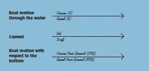
Figure 17-23 Just as lines are plotted on a chart, the DR current diagram must always be carefully labeled. Direction is shown above the line and speed below.

A study of the effects of current resolves itself into two basic situations. The first situation occurs when the set of the current is in the same direction as the boat’s motion, or is in exactly the opposite direction. In the second situation, the direction of the current is at an angle to the boat’s course, either a right or an oblique angle.

The first situation is the simplest to solve. The speed of the current—the drift—is added to or subtracted from the speed through the water to obtain the speed over the ground. The course over the ground (or intended track) is the same as the DR course—COG equals C, as does TR.

Since a GPS receiver shows course and speed over the ground, a boater need not calculate the effects of current set and drift as long as GPS is working correctly. But the wise navigator will know how to solve current diagrams in order to predict such effects ahead of time (and their likely impacts on courses made good and ETAs) and as a hedge when the electronics stop working.

When the boat’s motion and the set of the current form an angle with each other, the solution for the resultant course and speed is more complex, but still not difficult. Several methods may be used, but a graphic solution using a VECTOR CURRENT DIAGRAM is usually the easiest to understand.

The accuracy with which the resultant course and speed can be determined depends largely on the accuracy with which the current has been determined. Values of the current usually must be taken from tidal current tables or charts, or estimated by the skipper from visual observations.

Basically, a vector current diagram represents the two component motions separately, as if they occurred independently and sequentially—which, of course, they do not. These diagrams can be drawn in terms of velocities or distances.

“Velocity” has a more detailed meaning than “speed,” since it is speed in a given linear direction, at a timed rate and within a frame of reference. The diagrams in this text will graph motions in terms of their velocities.

Such diagrams may also be called “vector triangles of velocity.” The term “vector” in mathematics means quantity that has both magnitude and direction—directed quantities. In current sailing, the directed quantities are the motions of the boat and the water (the current).

A vector may be represented graphically by an arrow, a segment of a straight line with an arrowhead indicating the direction, and the length of the line scaled to the speed; see Figure 17-24. If we specify that a certain unit of line length is equal to a certain unit of speed—that one inch equals one knot, for example—then two such vectors can graphically represent two different velocities. Any speed scale may be used, the larger the better for accuracy. However, the size of the available paper and working space will normally control the scale.

Vector current diagrams may be drawn on a chart either as part of the plot or separately. If drawn on plain paper, it is wise to draw in a north line as the reference for measuring directions.

Since boats are subject to two distinct motions—the boat through the water, and the water with respect to the bottom—we will now consider how the resultant motion, or vector sum, is obtained by current diagrams.

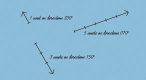
Figure 17-24 A vector has direction as shown by the arrowhead. It has magnitude as shown by its length. Both are referenced to a convenient scale.

When the two motions are not in line with each other, they form two sides of a triangle; see Figure 17-25. Completing the triangle gives the third side, which will be a vector representing the resultant motion or velocity. Consequently, when any two velocity vectors are drawn to the same scale and form the sides of a velocity triangle, the third side will be the resultant velocity vector (the vector sum of the other two), and its direction and magnitude may be measured from the diagram.

It may be easier to visualize the component motions if a time period of one hour is used and the points that are the corners of the triangle are considered as positions of the boat before and after certain motions, as follows:

• “DR”—the DR position of the boat as a result solely of its motion through the water.

• “W”—the position of the boat solely as a result of the motion of the water.

• “P”—the position (intended or actual) of the boat as a result of the combined action of the component motions.

It should be noted that although in some cases two of the above letters are applicable to a position, it is customary to use only one.

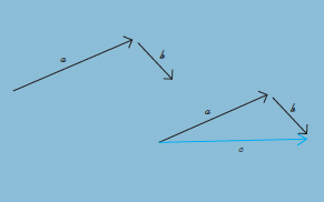
Figure 17-25 Vectors may be combined—their quantities added—graphically. In this sketch, vectors a and b are added, and their sum is vector c. The sum vector can be measured for both magnitude (length) and direction in the same manner as you would measure a line on a chart.

Note carefully how the vectors, one representing current and the other the boat’s motion through the water are drawn “tail-to-head.” (This rule applies only when one of the vectors is current, not when both represent the boat’s motion.)

If a boat's motion through the water (vector a) and the current's set and drift (vector b) are both known, either may be drawn first from the origin. In Figure 17-26, drawing A and drawing B both yield the same result for vector c.

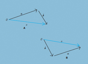
Figure 17-26 Vector diagrams A and B appear to be different because vectors a and b have been drawn in reverse sequence. But the sum, c, is the same in both instances.

There are four typical current problems, designated for convenience as Cases 1, 2, 3, and 4.

• Case 1: What is the set and drift of an unknown current from observation of its effect?

• Case 2: What is the effect of a known current if no allowance is made for it while running a DR course?

• Case 3: What is the corrected course to be steered, without regard for the effect on speed or estimated time of arrival?

• Case 4: What is the course and speed to arrive at a specified time? This is the “rendezvous” or “contest” case; see Figure 17-27.

We will run through each case three times: first using the traditional tools and skills of piloting; second using GPS; and finally using a chartplotter.

Figure 17-27 Proceeding toward a rendezvous point, this skipper compensates for the effect of current by adjusting his course and speed so that he arrives at his destination at the desired time.

CASE 1: DETERMINING CURRENT SET & DRIFT

This is a situation in which you know the course you have steered and the speed through the water from either the speed curve of your boat or a marine speedometer. It is also obvious to you that you did not arrive at your DR position. From your chart plot, you have been able to determine the course and speed over the ground. Current has acted to set you off your course—you desire to know its set and drift.

After again drawing a north reference line, plot vectors for your motion through the water—C 255°, S 12 knots, and your motion with respect to the bottom—COG 245°, SOG 13.4 knots. These vectors are both drawn outward from the origin, O, to points DR and P respectively. The “tail-tohead” rule is not applicable, as neither of these vectors represents current.

The action of the current has been to offset your boat from DR to P (which is also point W in this case); thus the set is the direction from DR toward P, and the drift is the length of this line in scale units. In the diagram, the current is found to be setting 192° with a drift of 2.6 knots. This is the average current for the time period and the location of the run from O to P for which the calculations were made; it is not the current at P. For the next leg of your cruise, these current values can be used as is, or modified as required by the passage of time and/or the continuing change in position of the boat.

If you’re navigating with GPS or a chartplotter, the Case 1 scenario could proceed as follows:

Case 1 with GPS. As above, you steer 255° true at a speed through the water of 12 knots, winding up at position P rather than DR.Your GPS receiver gives you the lat/lon coordinates of P, and it also gives you the bearing and distance of DR (which you programmed into the receiver as a waypoint) from P. The receiver will display the bearing of DR in degrees true, degrees magnetic, or both, and the reciprocal of that bearing (in degrees true) represents the current set. The distance of P from DR, when referred to a 1-hour elapsed time, is the current drift. For example, if the distance of P from DR is 1.3 nautical miles after a run of 30 minutes, the average current drift during the run from O to P was 2.6 knots. No vector plotting is necessary.

The prevailing current (actually the net effect of all offsetting influences) can be found graphically by plotting vectors for the DR track of the boat and its actual course and speed for a given time, then adding the vector from DR to P.

Case 1 with chartplotter. You steer 255° true at a speed through the water of 12 knots, winding up at position P rather than DR. Your chartplotter displays your boat’s position with an icon at P on a digital chart, and gives you the lat/lon coordinates of P. If you pause the cursor over DR, it gives you the bearing and distance of DR, from which you can derive current set and drift as with GPS. There is no need to program the coordinates of DR into the chartplotter as a waypoint; simply pause your cursor over DR’s charted location.

Using GPS or a chartplotter in this fashion is easier and more convenient than vector plotting, but it is also an unlikely use of GPS or a chartplotter. There is no reason to diverge from an intended track—and perhaps wander unwittingly into hazardous waters--when you can rely on GPS or a chartplotter. Cases 3 and 4 below will make this clear.

CASE 2: FINDING THE EFFECT OF CURRENT ON A BOAT’S COURSE & SPEED

If the set of the current and the boat’s course through the water are as shown in the diagrams in Figure 17-26, then the boat will be set off to the right of the direction in which it is being steered.

We will use a current diagram (shown at right) to determine the exact extent of this effect; we will also determine the path that the boat can be expected to follow, as well as its speed along that path (in other words, the intended track and speed of advance), given a boat speed through the water of 10 knots and a current set of 130º and drift of 3 knots.

We first draw in a North line as a reference for measuring directions in the diagram, and then the vector for the boat’s speed through the water, O-DR, a line drawn from the origin in the direction of 070° for a length of 10 units. Next, we add the vector for current, DR-W, three units in the direction of 130°. Note that we have observed the “tail-to-head” relationship rule. (Either of these two vectors could have been drawn first; the triangle would appear differently, but the result will be the same.)

Because these vectors form two sides of a triangle of velocities, the third side, O-W, is the resultant velocity at which the boat moves with respect to the bottom under the combined influences of its propulsion and the current. The point W can now be relabeled “P.” The intended (or expected) track (TR) and the speed of advance (SOA) can be measured from the O-P line.

In this example, the results indicate that the boat can be expected to sail a course over the ground of 083° and to have a speed advance of 11.8 knots. Bear in mind that the directions of these vectors are plotted as true directions.

Summarizing briefly, we have drawn vectors to indicate independently the motion of the boat from two different influences—that of its own propulsion and that of the current. Actually, of course, the boat will not go first from O to DR and then on to P. All the time, it will travel directly along the intended track O-P. The boat is steered on course C, the direction of O-DR, but due to the effect of current, it is expected to travel along the intended track O-P. This is the intended route that must be considered for shoals and other hazards to navigation.

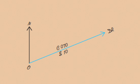
The north reference line is drawn first but is not needed if the diagram is plotted directly on a chart. This shows the vector line for the course and speed.

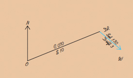
The vector for current set and drift is added; note the “tail-to-head” relationship of this second vector to the first one.

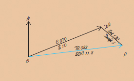
The connecting vector from O to P shows the resultant motion and speed of the boat over the bottom.

Case 2 with GPS.With GPS at your disposal, you can ascertain the effects of current on your boat’s course and speed without having to calculate the expected current from the Tidal Current Tables. Having programmed your intended destination, DR, into your GPS receiver as a waypoint, you start your run toward DR on a course steered of 070° at a speed through the water of 10 knots, monitoring your course over ground and the bearing to DR on the GPS display as you go. The initial bearing to DR is 070°, but the receiver may tell you that your course over ground is 083°, not 070°, and your speed over ground is 11.8 knots. You have learned this quickly, accurately, and without having to plot vectors. This is no reason not to have a handle on the local set and drift of the current, however. Without such knowledge you are blindly following an electronic black box—and that’s never wise.

If you continue to steer a course of 070°, the bearing to DR will soon begin to change—to 069°, then 068°, etc.—and the cross-track error function on your GPS receiver will show that you are diverging more and more from your intended track. To prevent this, you must alter course to compensate, as in Case 3 below.

Case 2 with chartplotter. If you are navigating with a chartplotter that is receiving GPS input (or with navigation software on a laptop that is interfaced with GPS), you don’t even have to program the intended destination, DR, as a waypoint. Simply begin your run toward DR and watch your boat’s progress across the digital chart. Pause the cursor over DR to note its bearing, and read your COG and SOG from the chartplotter display.

CASE 3: A TYPICAL CRUISING SITUATION

Here you know the track you desire to make good (TR 080°), you have decided to run at your normal cruising speed through the water (S 10 knots), and you have calculated (or estimated) the current’s set (140°) and drift (4 knots). What you desire to know is the course to be steered (C) and the speed of advance (SOA), which can be used to figure your estimated time of arrival (ETA).

Draw in a North line and measure direction from it (see the diagram below). Plot the current vector OW, at the specified direction and length, and a line (not a vector yet) from O in the direction of the intended track—this line should be of indefinite length at this time. From point W, swing an arc, with dividers or drawing compass, equal in length to the speed through the water in scale units. The point at which this arc intersects the intended track line is point P, and the vector triangle has been completed.

The direction of W-P is the course to be steered (C 060°); the length of the vector O-P is the speed over the ground (SOA 11.4), and from this the ETA can be calculated.

Let us look at the reasoning behind this graphic solution of Case 3. Again considering the component motions separately for the sake of simplicity, the boat is moved by current from O to W. It is to move from W at the specified speed through the water, but must get back on the intended track line—the problem is to find the point P on the track that is “S” units from point W. The solution is found by swinging an arc as described above. Remember that all vectors are plotted as true directions, including C, the course to be steered in the preceding solution. This must be changed to a compass direction (course) for actual use at the helm.

The DR Track

In accordance with the principles of dead reckoning, it is desirable to plot the DR track even though a current is known to exist.This line, drawn from point O in the direction C and with a length of S scale units, forms a basis for consideration of possible hazard if the current is not as calculated or estimated.

Case 3 with GPS. With GPS you can do more than ascertain the effects of current on your boat’s course and speed without having to estimate the expected current or calculate it from the Tidal CurrentTables, as in Case 2. You can also take the next logical step and correct for those effects.

At position O, enter your intended destination, P, into your GPS receiver as a waypoint, and the receiver gives the bearing of P as 080°. Accordingly you start your run toward P on a course steered of 080° at a speed through the water of 10 knots, monitoring your course over ground and the bearing to P on the GPS display as you go. Because the current is setting you to the right of your intended track, your COG will be greater than 080°, and the bearing to P will begin to change—to 079°, 078°, etc.To prevent this, you alter course to port until your COG is 080°—directly toward P—at which point you are steering 060° through the water. You are now proceeding crabwise, with your bow pointing well to port of P to compensate for the current.

Now that you’re heading toward P, you can read your speed over ground from the GPS display—the vector sum of boat speed and the effects of current—and find it to be 11.4 knots. You can also read your ETA for destination P.

If current set or drift should change as the run toward P progresses, you will detect this (provided you are monitoring the GPS) in a renewed cross-track error, and can correct as necessary.

If you were to proceed from position O on a course steered of 060°, failing to correct for current, your GPS receiver would display a progressively wider cross-track error, meaning that you were diverging more and more from your intended track. If you have programmed your receiver’s cross-track error alarm function, it will sound an alarm when you reach a preset error limit.There is an obvious safety value in presetting the alarm at less than the half-width of safe water in the alleyway along which you are proceeding.

Case 3 with chartplotter. If you are navigating with a chartplotter that is receiving GPS input (or with navigation software on a laptop that is interfaced with GPS), you don’t even have to program the intended destination, P, as a waypoint. Simply begin your run toward P and watch your boat’s progress across the digital chart. Pause the cursor over P to note its bearing, and adjust your course steered until your COG matches that bearing. If you don’t get around to this until your COG has diverged substantially from your intended track, a look at the digital chart will tell you whether your cross-track error has inadvertently placed a charted hazard (say, an isolated half-tide ledge) between your present position and P. If it has, the chart will also tell you how to detour around that hazard.

Like a GPS receiver, the chartplotter will display your SOG and your destination ETA. There is no vector plotting and no guesswork until the electronics malfunction and you need to fall back on traditional piloting skills.

If you know your desired track, and your speed through the water, agraphic solution can be used to determine the course to be steered and the speed of advance. For safety, aDR plot is added.

CASE 4: RENDEZVOUS

This is a variation of Case 3, in which you want to arrive at a specified point at a given time. It may be that you are competing in a predicted log contest, or merely that you have agreed to meet friends at that time and place. In addition to the data on current that you have, you have decided upon your track and your speed of advance. In the diagram at right, let us assume that the current sets 205° at 3 knots.You need to make good a track of 320°, and a quick speed-distance-time calculation sets your required speed of advance at 11.5 knots.

From the north reference line, draw the current vector O-W and the intended track vector O-P. Complete the triangle with the vector W-P, which will give you the course to be steered (C 332 True) and the speed to run through the water (S 13.0) to arrive at the destination at the desired time. Line O-DR should be drawn in from the origin as a dead-reckoning track for the sake of safety.

Case 4 with GPS. Having input waypoint P into the GPS receiver, you read the bearing of P (320°) on the GPS display and set out from O on a course of 320°. A southwest current sets you to the left of your intended track, however, so you alter course to starboard until your COG is 320°, at which point you are steering 332°. Then you adjust your throttle until your ETA matches the desired time, at which point your speed through the water is 13.0 knots and your speed of advance is 11.5 knots.

Case 4 with chartplotter. Proceed as with GPS, except that you don’t need to input P as a waypoint, and you can watch your progress across the digital chart. If you’re used to plotting current vectors, this is so easy it feels like cheating.

This problem concerns the course to be steered and the speed at which to run in order to arrive at a specified destination at a predetermined time. This could be used in establishing a rendezvous with another boat or in predicted log or other navigation contests.