
Before getting too deep into making adjustments to the running air/fuel ratio of the engine, it’s a good idea to take some time to understand exactly how the fuel injector works and is controlled by the ECU. In Chapter 4, we examined how the ECU determines the instantaneous airflow of the engine. The next step is to take the calculated aircharge and correctly convert this to the matching fuel charge. Fundamentally, this means calculating the pulsewidth, or time of injection for a single shot from each fuel injector. Not only must the ECU decide how long to leave the injector open, but it must also decide when to begin or end this cycle relative to the crankshaft position. Timing of the fuel charge delivery against intake valve opening time can have a noticeable effect upon engine torque, fuel economy, and smoothness.
First, let’s take a look at the window of opportunity to get the fuel into the engine. It takes some amount of time to flow a fixed mass of fuel through an open injector. The actual time required depends upon the flow rate of the injector and the pressure in the fuel rail that’s trying to push this fuel through the injector. We can also look at the engine’s cycle and know that the intake valve opens once every other revolution for the intake stroke. The faster the engine is turning, the more often the intake valve is opening or, more appropriately, the less time there is between intake events.

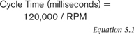
Cycle time for the engine decreases exponentially with speed, leaving less time for the injection event near redline. At idle, the cycle time is relatively large, so injector duty cycle is almost always a very small fraction.
The time available to get all of the necessary fuel into the cylinder along with the aircharge is equal to the cycle time for the engine. Cycle time is how long it takes for the engine to make two complete revolutions, with a single intake valve opening event per cylinder. The maximum available window of opportunity for fuel injection is therefore determined by the engine speed:
If the available cycle time for the engine is known, then the injector “on time” can be compared against it to find out just how much of the injector and driver capacity is being used at any given time. The injector duty cycle is defined as the ratio of on time to cycle time, usually expressed as a fractional percent:


For example, an engine operating at 3,500 rpm has a cycle time of 120,000/3,500, or 34.3 milliseconds (ms). If the ECU calculates an injector pulse of 6ms, then the duty cycle can be calculated as 6/34.3, or 17.5%.
An important note here is that there is no way for the ECU to execute pulsewidths that are greater than the cycle time. If a pulsewidth of 22 ms is commanded at 6 000 rpm (where the cycle time is only 20 ms), the result can only be an actual 20 ms pulse that is immediately connected to the following 20 ms pulse without any “off time.” Since there is no way for the ECU to magically add more time to the engine cycle, there is no such thing as 101% duty cycle in actual injector operation. The ECU may request it, but the physical speed of the engine dictates that the window is only so big and the most that can be done is continuous operation without interruption.
This is bad for two reasons. First, the necessary fuel is not being completely injected on each intake stroke. The result is a leaner air/fuel ratio than the operator desires and the ECU intends to deliver, which may lead to knock or more severe engine damage under high load. Second, the electrical transistors on the board of the ECU are being driven at 100% of their capacity without any rest. This puts a lot of current and ultimately heat through them, which may damage the drivers over the long term and render the ECU inoperable.

Many standalone controllers are offered in either batch or sequential injection configuration. The more advanced units like this F.A.S.T. are able to select either configuration from a menu as highlighted here.
The ECU must time the injection events to the engine’s rotation somehow. There are two primary strategies for doing this. The most primitive method is called “batch” fuel injection. A more advanced system known as “sequential” injection is the industry standard today. Each strategy has its own merits and limitations to either the ECU manufacturer or engine calibrator.

Marine engines are often equipped with central injection systems that are configured for batch injection. Boats are almost the ideal candidates for standalone EFI systems due to their simplicity in layout and wiring.
Batch fuel injection is the simplest form and easiest to implement with regard to software and ECU hardware design. With batch injection, groups of fuel injectors are all fired simultaneously for equal amounts of time. The groups usually consist of an entire engine bank of cylinders, so some manufacturers refer to this as “bank to bank” injector timing. However, the groups may be split across actual engine banks if the firing order of the injectors and cylinders are mixed. A four-cylinder engine with batch fuel injection will fire all of its injectors simultaneously while a V-8 engine will be split into two groups of four that alternate injection events. Actual injection time on a single batch or bank of injectors is typically split in two to provide one injection per engine revolution, but the total need only be calculated every cycle (two revolutions).
Batch injection simplifies the tasks to be performed inside the ECU since only one injection command must be calculated for each group of injectors on an engine cycle. The lower frequency of injection event time calculations means that a less powerful ECU can control the same engine to the same speed. On the other hand, a much higher revving engine can be controlled in batch fire since the processor load is greatly reduced. Additionally, ECU hardware costs are reduced since there are fewer required injection drivers on the board in order to control the same number of total fuel injectors.
The timing of the actual injection event on any given injector is not precisely aligned to each individual intake valve opening event. As such, there is no need to have precise camshaft-to-crankshaft- location detection. Fuel injected in batch firing is simply added to the intake manifold where it is allowed to freely collect upon port walls and evaporate as airflow and temperature dictate. In most cases, fuel is being added to the intake manifold at the same rate it is being consumed by the intake valves and cylinders, so a constant flow system is established. Occasionally, some cylinders will get slightly more or less fuel than desired, but on the average, desired conditions are met by the fuel delivery.
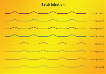
Batch fuel injection fires each injector once per crankshaft revolution as part of a group. Because the injection events are more frequent, the actual injection time is individually smaller and the timing of each event is not necessarily ideal.
Batch fire systems do not require that the fuel injector be installed close to the intake valve. It is common to see this strategy used in central-port-injection configurations that often look much like an electronic carburetor. If a system such as this is installed on the vehicle, batch injection is actually the preferred method of control.
The main drawback to batch injection is the lack of transient fuel control. If a rapid change in throttle angle is performed by the driver, the sudden increase of airflow will evaporate a larger part of the wall film of fuel that has been established by the system. Since the cylinder is depending on this wall film for a very large part of the total fuel mass delivery, the cylinders may exhibit a momentary lean condition. Much like a carburetor, a large accelerator pump function must be built into the software to offset this. The opposite is also true during a throttle closing event, usually leading to an excessively rich condition that may load up the engine if left unchecked. Tuning this transient fuel delivery can be tricky since the amount of correction needed changes with temperature and airflow.
Sequential fuel injection breaks down the timing of injection to a cylinder-by-cylinder chain of events. The ECU is given a specific order in which to fire the injectors, which is identical to the firing order of the engine. A single pulse is calculated for each injector that is timed to end at a specific interval before the intake valve opens. This allows for much more precise metering of the fuel being delivered to a given cylinder cycle.
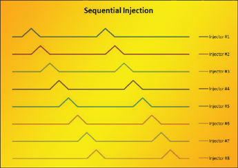
With sequential fuel injection, each injector fires only once per engine cycle (two crankshaft revolutions). The order of the injectors can be mapped to the firing order of the engine to make each injection event precede the intake valve opening on that cylinder.
The ECU must be properly equipped to handle sequential injection. Truly sequential operation requires a single driver for every injector as well as some method of detecting engine position and phase. Recognizing engine speed is typically done with a crankshaft sensor, but a camshaft sensor must also be installed to distinguish between TDC events for intake and power strokes on a given cylinder. Without this, the best the ECU can do would be a blended “staged sequential” operation that fires pairs of opposed injectors once per revolution. While mildly better than batch fire, it still lacks the precision of a true sequential setup. Sequential injection also uses more processor time to run the engine as each injection event is calculated. All things being equal, this requires a faster processor to operate the same engine at the same maximum RPM, which may increase the cost of the ECU. Fortunately, it’s not hard to come by very affordable processors with sufficient speed for sequential fuel injection operation these days. The real trick is having the necessary software and board outputs to execute the strategy.
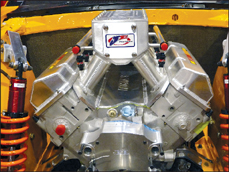
Dedicated race engines that operate at high RPM and airflow rates are better suited to batch injection. If the injection pulsewidths are large, the starting and ending point of each event get closer together.
Sequential fuel injection requires that the injector be installed relatively close to the intake valve for best results. The small amount of “wet” intake port area means that a larger percent of the fuel entering the cylinder comes directly from the injection event instead of evaporation of the wall film. This more precise control of total delivered fuel mass on each intake event gives the ECU better control during transient throttle conditions.

If idle stability and emissions are priorities, sequential injection timing can help. Just about every OEM system today includes sequential injection, which only helps the aftermarket performance when the modifications start.
The injection event can be timed so that it ends just before the valve opens. This reduces the chances of the fuel that was meant for that particular cycle going anywhere else. By injecting against a closed intake valve, most of the fuel is quickly evaporated and a cloud of fuel vapor is available for intake immediately as the valve opens. This promotes good mixing of the fuel charge within the cylinder and allows more of the fuel to burn closer to the desired ratio. Unevaporated fuel can lead to pockets of richness and leanness within the cylinder that burn unpredictably and poorly. The combination of properly timed injection events and smaller “wet” intake port area leads to a significantly reduced need for pump shot or acceleration enrichment. Individual cylinders can even be tuned to offset airflow differences in the intake manifold so that each cylinder operates at the desired air/fuel ratio at all times. OEM engineers have long recognized these benefits and it’s the reason why every car today uses sequential injection from the factory to improve emissions and overall engine performance.
There are two types of fuel injectors commonly used today. The biggest difference between them is the impedance of their internal circuits and, consequently, how the current is applied to the coil.
Most OEM vehicles today use high impedance (12 to 16 Ω) injectors. According to Ohm’s Law, the higher resistance dictates that the current will remain low. Low operating current means less heat in the wires and ECU board traces that power the injector, which is good for durability. The ECU signal that opens the injector looks like a square wave function that discretely switches on and off.
High impedance injectors are often referred to as “saturation” type injectors. The name comes from the electrical function of the driver. High-impedance injector drivers simply turn on and stay on for a predetermined amount of time. Once turned on, it takes a small amount of time to completely energize the coil inside the fuel injector. Naturally, this time delay between initialization of current flow and actual fuel injector pintle movement must be taken into account by the ECU. Although it is not a tremendously large amount of time, it is still significant, especially when compared to the desired flow times at idle. The fuel injector coil is driven to saturation, and held under this condition for as long as the ECU intends the fuel to be flowing.

The difference in current profiles for high impedance (saturation) versus low impedance (peak and hold) is significant. If low impedance injectors are installed with a saturation driver in the ECU, the current will remain high for the entire injection pulse, which may damage the ECU.
Upon completion of the desired flow time, current through the injector driver is shut off. Because the coil is still saturated (there is some amount of inductance), the injector does not close until the field can collapse and the force holding the pintle open disappears. Again, this is a very small slice of time that must be accounted for by the ECU.

It takes a small amount of time for the electrical energy from the ECU to overcome the resistance of the injector’s closing spring and fuel pressure before actually opening for fuel flow. This delay time varies with injector design and can represent a significant portion of the idle pulsewidth.

Injector opening time varies with system voltage and can differ significantly compared to normal idle pulsewidths. This table is not accessible for recalibration on all ECUs, but it should at least exist in the background.
The difference between the opening delay and closing delay is known as the injector offset. The injector offset is the value that the ECU will add to whatever desired flow time is calculated for the injector on a given shot. If this time offset is not used, the actual fuel delivery would be lower than desired, resulting in a lean condition. Since the time offset is relatively small, this is most noticeable at low pulsewidths near idle where this offset represents a significant percent of the total open time. Most high impedance injectors have a combined injector offset of approximately 0.4 to 0.8 ms at normal vehicle operating voltage. If a total idle pulsewidth of 2.0 ms is calculated based on airmass and injector flow rate and the offset is 0.5 ms, we can see that 25% of the energization time of the circuit is just dedicated to getting the pintle open in the first place. This can be the difference between a lean misfire condition and an engine purring at an idle fuel mix of lambda=1.00.
The injector offset is a function of available voltage. Higher voltage means more energy available to quickly saturate the injector coil and open the pintle. The relationship between available voltage and injector offset times for a typical high impedance injector can be seen above. Although the changes to injector offset are relatively subtle at and above normal operating voltage, any time voltage drops, a significant adjustment can and should be made to injector pulsewidth to compensate for the change in offset. Something as simple as a weak battery during cold cranking that only has 9 volts available can require an entire extra millisecond of additional on time for the injector just to get the same fuel mass delivery as seen under normal conditions. Further, you don’t want a failed alternator, which results in low system voltage, to render the engine immobile due to an excessively lean condition. If the injector offset is properly compensated for a wide range of system voltages, at least the delivered fuel mass will remain on target if other unfortunate circumstances arise.
The other common type of fuel injector is the low impedance or “peak and hold” variety. These injectors have a significantly lower internal impedance of approximately 2 to 6 ohms. As expected, the lower impedance of these injectors leads to a generally higher operating current, so the proper changes must be made to the ECU injector driver hardware prior to using these.
The name “peak and hold” comes from the function of the injector driver used to control these low impedance units. The low resistance coils are easily excited to full field potential and do not require as much energy to maintain this field throughout the remainder of the injection pulse. Once the field has been established and the injector is open, current through the coil is reduced to a nominal amount and held there until the end of the injection event. Closing times are also much shorter since there is less inductive energy to dissipate after the driver is shut off. Typical injector offset time for a low impedance unit is approximately 0.2 to 0.4 ms.
The primary advantage of the low impedance fuel injector is the significantly shorter injector offset times that are possible. Shorter and more consistent injector offsets mean that the ECU can reliably control much shorter pulsewidths. This becomes extremely helpful when the static flow rate of a fuel injector is relatively high. The higher the static flow rate, the shorter the pulsewidth needed to supply the same amount of fuel. If the flow rate is too high, it may become impossible to deliver a short enough pulse to deliver the small fuel amounts required at idle. Low impedance fuel injectors alleviate this problem by giving the ECU more control in this range.
Most OEM applications can be satisfied with fuel injectors whose flow rate is low enough to allow the use of high impedance injectors and still maintain sufficient idle control. As such, there is no reason to justify the added expense of the peak-and-hold drivers. Luckily, most aftermarket ECUs are built knowing that there is a good chance the user will attempt to make more power than the typical OEM application. Standalone ECUs are typically equipped with peak and hold injector drivers that can handle almost any port fuel injector out there.
On the most basic level, total fuel flow is directly proportional to the pulsewidth. The longer the injector is held open, the more fuel is injected and available for intake when the valve opens to the cylinder. The rate at which fuel is delivered through the open injector is often referred to as the “size” of the injector, such as 42 lb/hr. Since many fuel injectors are mechanically interchangeable, what is really of note here is the flow rate or slope of the fuel injector.
The graph on page 43 shows the actual fuel mass delivery over time for a single shot. It is important to note that the axes for this graph show fuel mass and time. Earlier, I noted that the ECU works in terms of airmass and fuel mass. The relationship shown in this chart is what the ECU uses to convert from the calculated fuel mass desired to go with the airmass into an injection time that will be passed to the driver circuits. The opening delay is clearly visible as the vertical gap starting from time zero. Once the pintle is actually opened, one can see a straight-line relationship between time and fuel mass. It is the slope of this line that is most often used to describe an injector “size.” The injector’s upper slope of the fuel mass delivery is more appropriately known as the static flow rate. The algebraic definition of slope is rise over run. So in this case, the rise is accumulated fuel mass and the run is time. Fuel mass over time gives us the more familiar units of pounds per hour or grams per second that we are used to seeing when describing injector size or flow rate.

Most factory ECUs are equipped with saturation drivers that can only operate high impedance injectors. Using an external driver box like this one allows the ECU to still see the proper load while operating the low impedance injectors from its own power supply based on the signal from the original controller.
Shorter total pulsewidths are more significantly affected by the nonlinear flow rate that comes with a pintle that is only partially open for a significant amount of the total injection time. During the split second of injector opening, pressure differential across the tip of the injector is at its highest. Once flow is established, the local pressure immediately behind the pintle relaxes slightly and the flow rate settles into the previously discussed static flow rate. The slope during this short window of high injector flow is known as the dynamic flow rate and can be approximately 10 to 15% higher than the static flow rate.
In a way, fuel injectors behave just like the average garden hose. Water is turned on at the faucet with a nozzle attached to the end of the hose. The hose itself behaves like the fuel rail in an engine, retaining some pressurized reserved supply that can be delivered by opening a valve at the end. Opening the nozzle on the hose is similar to the ECU triggering the fuel injector. Immediately upon opening, the water stream shoots the longest stream possible and quickly recedes to a lower, but still very sizable, flow. The distance at which the water lands from the user holding the nozzle is proportional to the available water pressure. Since the flow area of the nozzle is constant when completely open, it is safe to say that this increase in water pressure has delivered an increase in water flow rate. Flow rate is then represented by the landing distance of the water stream. The longer initial distance is proof that the flow rate was temporarily greatest immediately after opening the nozzle. The same happens each time an injector is fired. A slightly higher flow rate is realized for a very short duration before static flow is established.
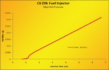
The actual fuel delivered over time for one particular injector. This unit stabilizes to a slope of 5.26 grams per second or about 41.7 lbs/hr.
The best control systems will have more elaborate injector flow modeling capabilities that can accurately represent this phenomenon. This can be done by either shifting the desired pulsewidth of the injector based on some reference table or by providing two different injector slopes for static and dynamic flow rates. If neither compensation strategy exists in the ECU, any fuel delivery errors in the low flow range will simply be “baked in” to future airflow calculations in order to maintain a stable air/fuel ratio near idle and light load conditions. In a speed density system, this would show up as slightly increased values for volumetric efficiency in the low load region, even though the actual flow may be lower.
Ohm’s Law and Fuel Injectors
V = I x R
Ohm’s Law states that voltage in a circuit is the product of current (measured in amps) and resistance (measured in ohms). If the voltage available in a circuit remains constant, then current must increase as impedance decreases to satisfy the equation. In the case of fuel injectors, the ECU operates with roughly 12v available. If we have a fuel injector with an impedance of 14 ohms, the current is then found by:
I = V / R
Or: I = 12v/14Ω = 0.857 amps, which is a fairly low current that is easily handled by most injector drivers. If a 2Ω low impedance injector is exchanged into the same 12v circuit, we find that the current increases significantly: I = 12 v/2Ω = 6.0 amps, an increase of 600% over the previous level. Since current flow is the primary contributor to heat and ultimately failure of these circuits, it becomes apparent that low-impedance-injector drivers built to handle these conditions are required. Running low impedance injectors on a standard (high impedance) driver will almost always lead to thermal failures, a damaged ECU, and a stranded vehicle. Always check to ensure what kind of injector drivers are included with the ECU before attempting to run the engine. If the ECU is not equipped to run low impedance injectors, an outboard injector driver box may be employed to avoid damage to the internal drivers of the ECU.
The static flow rate of a fuel injector can be used to estimate the maximum power that can be supported. It is also possible to decide what size injector is necessary based on how much power is expected. Both calculations are tied to air/fuel ratio and engine efficiency. The common measure of this is brake specific fuel consumption (BFSC), expressed in terms of grams per kilowatt hour or pounds per horsepower hour. Since most fuel injectors are listed in units of lb/hr, it makes sense here to depart from the metric system for an example.
Most naturally aspirated engines consume fuel at WOT with a brake specific fuel consumption somewhere between 0.3 and 0.5 lb/hp-hr. Supercharged engines, which run richer under high load, will be slightly higher at 0.55 to 0.7 lb/hp-hr. Using this basic efficiency unit, one can simply multiply the target maximum horsepower by anticipated BSFC to show total engine fuel delivery needs:

For example, a 500 hp supercharged engine operating at an anticipated 0.6 lb/hp-hr BSFC would need 300 lb/hr of total fuel flow. This represents the fuel being delivered to all cylinders combined, so it can be split across any number of available injectors. With one injector per cylinder, the minimum individual injector flow is found by:

In this example, a 500 hp V-8 engine using 300 lb/hr of total fuel flow would need an absolute minimum of 37.5 lb/hr static flow rate from each individual injector. Some may stop here and go out to purchase injectors for their 500 hp engine. This would be a mistake because the injector drivers in the ECU should not be run at full capacity on a continuous basis. Doing so will often overheat the transistors that drive the fuel injector from the continuously high current flow. To avoid this, some safety margin should be used to give the injector drivers a rest between shots. A 20% safety margin will usually be sufficient to prevent the overheating of the injector drivers. The safety margin is applied to the minimum injector flow rate. See Equation 5.5 below.

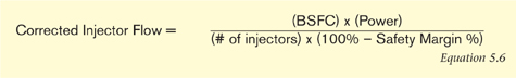
To continue our 500 hp V-8 example, the introduction of the 20% safety margin yields a corrected injector flow requirement of 46.9 lb/hr. This would mean that even at the engine’s maximum power output and fuel enrichment, there is still room left over for some extra flow. Combining Equations 5.3, 5.4, and 5.5 gives a single comprehensive equation for estimating injector size based on anticipated power and fuel consumption rates. See Equation 5.6 below.
The added safety margin comes in handy when the car may be occasionally run in cold weather where air density is higher, power is increased, and total fuel requirements are slightly higher than the original calculation assumptions. Otherwise, a car that is equipped with injectors that are barely adequate may run lean in cold weather, possibly leading to engine damage. A little extra safety margin here can save thousands of dollars and countless hours of later aggravation.
By now, it should be fairly obvious that increasing fuel pressure will increase the flow rate of any injector. Even better, it has been established that this relationship between pressure and flow is predictable. Because fuel injectors are effectively a fixed orifice for fuel flow when open, they follow the Bernoulli equation for pressure and flow rate:

This Nissan GTR requires significantly more fuel injector flow capacity to match the increased airflow capacity from the twin turbos. Turbocharged engines typically operate at richer air/fuel ratios than their naturally aspirated counterparts, which further drives the need for large fuel injectors.
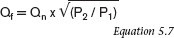
Here flow is represented by the engineering shorthand “Q,” where Qf is the final flow rate and Qn is a nominal or reference flow rate. Reference pressure is P1 and final pressure is P2. This equation can be used to compensate for changes in fuel pressure setting that are different from the rated flow pressure of a known fuel injector. Many fuel injectors are listed with static flow rates as tested with 3 bar (43.5 psi, 300 kPa) reference pressure. If this injector is used in an application where the static fuel pressure is different, it is imperative that the flow rate values entered into the ECU are adjusted. Failure to do so will result in skewed injection time calculations and often lead to improper adjustments to the airflow models and VE tables during the calibration procedure.
An example of the practical use of the Bernoulli equation would be the installation of a set of Bosch “green top” fuel injectors in a late model GM fuel system. The Bosch specification for these injectors is 42 lb/hr of static flow at 3 bar (43.5 psi). The GM fuel system is internally regulated to a pressure of 4 bar (58 psi), so one can naturally expect some increase in the flow rate. The new static flow rate is found by using Equation 5.7:

In order to give the ECU the best control of actual fuel delivery at this elevated fuel pressure, it’s a good idea to use the new value for injector flow rate of 48.5 lb/hr instead of 42 lb/hr. There is a 15% shift between the two, which can be the difference between starting out right on the target of 14.6:1 air/fuel ratio and 12.64:1 when first targeting lambda=1.00 at cruise. It is imperative that the fuel injector flow rates are correct, since they will be used as one of the key assumptions when calculating airflow corrections. The more accurately the injector flow is represented in the ECU, the more precise the calibrator can be later on when making changes to the VE table or other airflow calibrations.
The relationship between fuel pressure and flow can be used to the engine builder’s advantage. If a set of fuel injectors is just slightly undersized to support the desired engine power level and flow requirements, a calculated increase in rail pressure can be used to effectively increase the injector flow rate.
Our theoretical 500 hp V-8 engine requires a static injector flow of approximately 46.9 lb/hr. If the vehicle is equipped with a set of “green top” 42 lb/hr injectors, we can see that the engine runs the risk of running lean or overheating the injector drivers in the ECU. The fuel rail pressure can be adjusted upward to recover the safety margin. Using the above example, the 42 lb/hr fuel injectors effectively become 48.5 lb/hr injectors when the pressure is raised from 3 bar up to 4 bar. This 15% increase in flow capacity translates directly into an additional 15% more horsepower that can be supported at the same air/fuel ratio. More importantly, the increase in fuel rail pressure has brought the static flow rate above the corrected injector flow that correlates to our desired 20% safety margin even at the 500 hp level. This engine should have no trouble delivering the required fuel mass even under the most extreme conditions.
The fuel-pressure-correction math works both ways though. The pressure used in this equation is not absolute or even gauge pressure. It is really pressure drop across the injector itself. The measurement is usually taken with atmospheric pressure acting on the regulator’s diaphragm. This usually means either disconnecting the vacuum line from the intake manifold briefly or taking the measurement when the fuel pump is running and the engine is not. Most mechanical fuel pressure regulators will automatically hold a constant pressure differential between the reference side and the rail pressure itself. If the reference side is connected to the intake manifold by a vacuum line, the reference pressure will decrease when the engine is throttled at idle or cruising conditions. This lower reference pressure results in a similar decrease in rail pressure, keeping the pressure drop, or “delta,” across the injectors constant even as MAP changes. This is what ensures that the static flow rate of the fuel injector remains at the same value that the ECU is using for its own injection time calculations.
Even better, these mechanical regulators will almost always work when positive manifold pressure is applied. Each pound of manifold boost from a supercharger or turbocharger should be met with one pound of rail pressure increase to maintain a constant injector flow rate. As long as the fuel pump has the capacity to maintain this increased pressure at the necessary flow rate, everything works just fine. However, if for some reason rail pressure does not increase 1:1 with manifold boost, the flow rate of the injector is decreased. This drop in rail pressure delta may be a symptom of inadequate fuel pump supply or undersized feed lines and rails. Unfortunately, this is usually under high load and flow rate conditions, just when it is needed most.
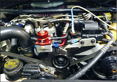
This adjustable fuel pressure regulator makes it easy to effectively change the flow rate of the fuel injectors. The vacuum line is connected to the intake manifold, allowing the regulator to maintain a constant pressure drop across the injectors even as intake pressure changes with throttle movement.
Continuing to use our theoretical 500 hp supercharged V-8 engine, let’s take a look at what happens if we make 10 psi of boost, but only see 40 psi on a fuel pressure gauge. Earlier, we intentionally moved the target rail pressure up to 58 psi delta. This delta is the difference between manifold and rail pressures. The addition of 10 psi of manifold boost means that we should really see 58 psi plus 10 psi, or 68 psi total guage pressure at the rail if we are to maintain the target flow rate. Since we effectively have a drop in available pressure across the injector, we can calculate exactly how much the flow rate has reduced as a result using Equation 5.7. In this case P2 (40 psi from the gauge) is actually lower than P1 (58 psi target), which will work out to give us a lower flow rate:

It becomes clear here that the reduced injector flow rate that results from the lower fuel pressure delta is lower than the original 42 lb/hr that did not have sufficient safety margin. In fact, it’s only slightly higher than the 37.5 lb/hr absolute minimum requirement at 100% output. Although this particular engine probably won’t drift lean under load, it still doesn’t have very much reserve for cold weather, high barometric conditions or other unforeseen load increases.
The solution here should be to investigate the cause of the dropping fuel pressure. This may be as simple as a clogged fuel filter that hasn’t been changed in a while. It may also be a sign that the fuel pump just can’t keep up with the flow requirements of the engine and injectors. A higher flow aftermarket pump will usually fix this at a modest cost penalty. Keep in mind that a fuel pump’s maximum flow capacity varies with total pressure. A fuel pump’s energy can be used to generate high pressure or high flow rates, but usually not both. It must trade one for the other at maximum output, so it pays to verify that the pump can support the necessary flow rate at the pressure needed to maintain the desired injector delta pressure.

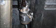
In a supercharged application, it’s important to consider intake manifold pressure as well as fuel rail pressure when determining injector flow rates. This Ford Mustang’s factory ECU is equipped with a sensor that measures the delta pressure across the injectors directly by sampling both fuel and intake pressure across the same diaphragm.
If the pump being used is advertised as being capable of supporting the flow rates in question, it may be time to look a little deeper at the vehicle hardware. On an otherwise stock vehicle, we may find that the relatively small diameter feed line between the pump and engine may be causing the restriction. Even though the fuel rail may be operating at 60 psi, there may be additional pressure drops between the rail and pump from the line and filter restrictions. Upgrade as necessary before attempting to fix any of this with ECU calibration adjustments.
Some aftermarket ECUs have the ability to control more injectors than the engine has cylinders. The simplest way to accomplish this is by simultaneously firing two equally sized injectors. The fuel mass is split evenly between both injectors on the same cylinder. This effectively doubles the power capacity of the fuel supply as long as the pump can keep up. The only drawback to this is that it also doubles the minimum amount of fuel that can be injected. This may make it difficult to control the small fuel mass requirements at idle and light loads.
If the ECU is able to discretely control two injectors per cylinder and time them independently, they can be configured so that only one injector fires per cylinder at low loads. At higher loads, where the single injector would be quickly running out of capacity to support the necessary fuel flow, a second injector on the same cylinder is triggered to share the fuel delivery. This is known as staged injection. The onset of the second injector contribution can be triggered by injector duty cycle, total instantaneous flow rate, or manifold pressure.
A clear advantage to staged injection is that the primary fuel injectors do not need to be tremendously sized in order to support a large amount of total engine power. The smaller primary injectors will then have correspondingly larger pulsewidths at idle and low rates. This longer pulsewidth makes it easier for the ECU to make very fine adjustments to total fuel mass deliveries. It also means that the injector offset represents a much smaller percent of the total on time during idle pulses. Again, this reduces the variability of air/fuel ratio control just when it is most critical. The end result is an engine system with tight control of delivered lambda and ultimately cleaner burning, better emissions, rapid throttle response, and superior fuel economy.
The fuel filter is often one of the more neglected parts on a vehicle’s maintenance schedule. A clogged or damaged fuel filter can reduce delivered fuel rail pressure at high load, leading to a lean condition that may damage the engine.
The only real downsides to staged injection are cost and complexity. Staged injection almost always required some rather exotic modifications to the intake manifold to provide the additional injector locations as well as fuel rails and lines to feed them. The ECU must also be manufactured with the additional output drivers and be programmed with the necessary code to divide the fuel mass delivery across two different injector groups. There are only a handful of OEM applications that allow for multiple injectors per cylinder for just these reasons.
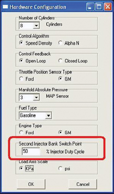
The BigStuff3 system allows the user to determine the turn-on point for the second set of fuel injectors. Here it is set so that once the first set of eight injectors reaches 50% duty cycle, the fuel mass will get split evenly across all 16 injectors to increase capacity at high loads.

Staged fuel injectors allow for better control where a single injector per cylinder is used for most light duty operation. This engine has a second fuel rail that feeds another pair of fuel injectors per cylinder for a total of three injectors per cylinder. That’s a lot of fuel to go along with those two huge turbos.