
Once the framework of the calibration has been established by properly setting up the sensor inputs, firing order, and injector constants, we can move along to what is arguably the most important table in the whole ECU calibration. The volumetric efficiency (VE) table is the ECU’s reference for pumping efficiency across all engine speed and manifold pressure conditions. Adjustments to this table have an effect upon almost every other aspect of ECU and engine operation, so it is imperative that this table is calibrated in the most accurate way possible. As discussed earlier in chapter three, the volumetric efficiency value taken from this table is used to infer an effective working cylinder volume that is in turn used to calculate the current cylinder airmass. Although VE is not the only variable in the airmass calculation, it is one of the most dominant. Volumetric efficiency is a direct multiplier upon calculated airmass, so a 10% change in VE yields a 10% change in calculated airmass.
Collecting the data to populate the VE table is a tedious process. When working with a complete engine and wideband to solve for VE, there are several serious concerns. First, one must understand that there is a very strong assumption of accuracy in fuel delivery. When adjusting VE based on measured lambda error, we are basically saying that all of the delivered error in air/fuel ratio is a result of improper airmass estimation. In doing so, we rely upon the fuel injector to act as a metering device. Here is where we begin to realize just how important it was to be as precise as possible when modeling the fuel injectors’ physical behavior in the ECU calibration. If the actual amount of fuel flowing through the injectors differs from what the ECU model shows, an error is introduced into the system. Left uncorrected, this error would get “baked in” to the VE table corrections. This error is usually most apparent at the low injection times associated with idle and light cruising conditions where some larger flow rate injectors have not yet reached the linear portion of their flow curves. The bigger the injector, the more likely this is to matter since their breakpoints before reaching steady flow tend to be numerically higher in terms of fuel mass. Just as important is to make sure that the linear flow rate of the injector really is in line with ECU expectations. Remember that something as simple as a change in expected fuel pressure can lead to a whole series of incorrect calculations here. One can rapidly see where the earlier efforts to accurately describe injector function to the ECU make the job of calculating VE easier, regardless of fuel flow.

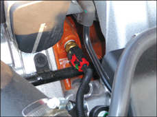
Before attempting to use a wideband to calculate corrections to an airflow model like the VE table, it is important to ensure that the injector characteristics are correct within the ECU. This also means verifying and carefully setting the fuel rail pressure to avoid errors due to the Bernoulli effect.
The second serious concern when working on a VE table calibration is consistency. Most notably, this means taking the data under the same conditions for all points in the map. The physics equations shown earlier that take us from PV=nRT to cylinder airmass are just as dependent upon temperature as they are upon volume. The 1/T function can skew the calculated airmass significantly if it changes during the course of testing. Since we are actually solving for relative volume in this case, it becomes necessary to hold temperatures as close to constant as possible. This means keeping a careful eye on both intake air temperatures and engine coolant temperatures. The actual temperature in question is the gas entering the cylinder, which is a function of both inlet temperatures and any heating or cooling that happens to the gases as they go through the intake manifold and cylinder head ports. If the engine is at normal operating temperature, the air entering the cylinders is almost certainly heated by some amount after it passes the throttle body. More sophisticated ECUs will even have a whole series of tables to describe the amount of aircharge heating as a function of engine coolant temperature and MAF rates. For simplicity, it’s best to just plan on starting your VE table measurements and adjustments with everything at a “normal” temperature. In practice, this means letting the coolant and the rest of the engine get up to normal operating temperatures before attempting to adjust the VE table. This minimizes the impact of the temperature influence on our adjustments. You can come back later and modify the temperature-based compensation if needed for a cold engine.
Monitoring engine coolant temperature is key during the population of the VE table. There are separate correction tables that can be used for extreme temperature compensation, so the VE table should be corrected only under normal operating conditions.
So where does one start with VE table population? The values need to come from somewhere. The easiest starting point is another calibration for a similar engine that is known to operate well. If someone else has already done the homework here, it’s a good idea to copy it in order to get a running start at what can be a very daunting task. Most popular engines have already been calibrated somewhere before, it’s just a matter of digging a little to find an example. In many cases, the manufacturer of the ECU may have a selection of reference files from which to start. Even if you are not using that exact hardware combination, one of these files can at least give you something to work from as you make the first attempts at quantifying volumetric efficiency.
If you decide to start with an existing VE table, don’t feel tied to the axis breakpoints or values shown. Remember that the key function of the VE table is to represent the physical pumping efficiency of this particular engine. Changes as subtle as muffler design, air filter housing, or header length can have significant effects upon the VE table in multiple places. Don’t be afraid to move RPM breakpoints on the table if it is an option on your particular controller. The reference engine may have idled at 900 rpm, but a milder camshaft in your application may allow you to settle to 650 rpm. If this is the case, you will certainly want breakpoints in the VE table directly on, as well as just above and below, your final target idle speed. This will afford the ECU more precision in calculating the cylinder airmass during one of the most critical and customer-sensitive engine functions. You don’t want a rolling idle to be exaggerated by inaccurate airmass calculations that could be prevented by increasing the table precision here. It is preferred to have breakpoints within no more than 200 rpm on either side of the warmed-up idle speed to give the best results.
On a similar note, make sure that the top values of speed in the VE table align with the expected RPM range of the engine. There is no use in having a VE table that extends to 9,000 rpm if the camshaft is only expected to perform up to 6,500 rpm. These extra cells of table resolution are better used at lower speeds where the pumping efficiency is more likely to change with speed. If, for some reason, the maximum engine speed in the VE table is exceeded, most ECUs will take the last value seen at the table maximum and continue using it until the engine returns to the table’s prescribed range. As long as the final engine speed breakpoint was beyond the torque peak of the engine, the result is usually only an overestimation of cylinder airmass and a rich fuel condition. This is definitely better than underestimating airmass (which would lead to a lean fuel condition at high speed), but is still not desirable. In short, make sure that the ECU tables match the engine hardware’s capabilities.
Remember what you just read about engine speed range in the VE table? The same goes for manifold pressure. Engines with large-duration camshafts will not typically have a very strong idle or cruising vacuum. As such, there is really no need to provide a whole array of MAP breakpoints below idle vacuum if the engine simply can’t get there. This resolution is once again better spent above idle MAP points where more precision can be given to tip-in conditions that are very sensitive to the driver. If the engine is boosted, it is absolutely critical that the VE table include breakpoints above 100 kPa to calculate the proper cylinder airmass. If the engine runs more than 14 psi of boost, the same holds true for exceeding the 2 bar MAP limit of 200 kPa. Just like with RPM, the ECU has no choice but to use the last known value for VE if measured MAP goes above the last breakpoint in the table. The potential results here are more concerning than just going beyond an engine speed breakpoint since adding boost typically increases relative airmass and any air/fuel errors at this level can be very costly.
If you simply don’t have any reference calibrations available to look at and copy, you’re in for a slightly more challenging time while calibrating. This doesn’t make it impossible by any stretch, just a bit more time consuming. In an absolute-worst-case scenario, the entire VE table would start out populated by the same number in every single cell, perhaps around 60% to begin. We know that the finished table will be anything but constant, but you have to start somewhere.
With some sort of values entered into the volumetric efficiency, an attempt can be made to run the engine. To begin, we will set the desired air/fuel ratio to a constant value across all speeds and loads. This will make the calibrator’s life much easier since he is no longer trying to hit a moving target. Stoichiometric operation should be the goal to begin, so set the entire table to lambda=1.00 or approximately 14.64:1 for gasoline. By doing this, the delivered lambda measurement from the wideband will represent the exact correction factor we need to apply to the VE table value in question. In the beginning, we will only be checking moderate loads, below 100 kPa, so no significant fuel enrichment is required. Later on, we can change the target air/fuel ratio for full load to a richer setting.
When the engine is first started, initial operation may be quite rough and unpredictable. If this is the case, the best course of action is to apply enough throttle to hold the engine at a higher speed. Approximately 2,000 rpm is usually sufficient to avoid stalling and help get the engine up to operating temperature quicker. Idle is actually very difficult for an engine to do properly and requires a fair amount of coordination between aircharge estimation, fuel delivery, and spark advance to hit a moving target while warming up. By skipping this step completely for the time being, one can focus on the easier task of quantifying part load VE where the engine is far more forgiving of delivered air/fuel ratios and timing changes. In reality, most engines will at least continue to operate at light loads and moderate speed even if the delivered air/fuel ratio is as rich as lambda=0.61 (9.0:1 AFR) or as lean as lambda=1.36 (20:1 AFR).
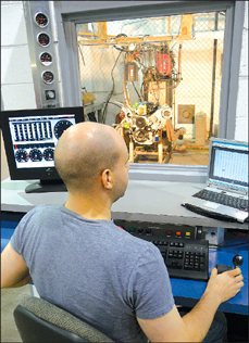
The engine dyno is the best tool for developing a VE table because the operator can simply dial-in whatever combination of engine speed and load he desires. Large cooling systems allow the engine to operate for long durations under conditions that would otherwise overheat a conventional radiator or vehicle cooling system.
If, during the initial checkout, a wideband reading of extremely rich or lean is consistently seen, it’s a good idea to make a global change to the entire VE table as long as there are no other mechanical problems such as air leaks or fuel delivery issues. Don’t be afraid to make what appear to be very large changes here. It’s not uncommon to need to make 30% or greater shifts when first tuning a new combination. In these preliminary steps, the changes are applied to the entire VE map since it is often difficult to tell exactly which cells are being used to calculate the current volumetric efficiency and airmass. Chances are, whatever physical changes to the engine that require a local change in VE, also require similar changes at higher speeds and loads. You will still get a chance to fine tune individual cells later if this first global shift proves too aggressive.
Carefully choosing the breakpoints for the VE table before starting can make the final calibration much more robust. Having more resolution at low speeds gives better idle control and tip-in behavior while upper RPM points can be spaced farther apart without much compromise.
At this point, the dynamometer should be configured to perform a constant speed test. Ideally it would be set to control to engine RPM, but a constant wheel speed test will also work. Vehicles with a manual transmission are easier to operate on a chassis dynamometer for this testing since they have a single fixed ratio between engine and wheel speed for each gear. Just pick a gear and drive the vehicle under moderate load on the dyno and allow the load absorber to control speed. Third or fourth gear usually works best since there is less gear multiplication and a more direct connection between the engine and driveshaft speeds. You will see that it’s easy to move between VE table load cells by simply moving the gas pedal. Applying more throttle angle will increase MAP and move vertically within the table at the same engine speed.
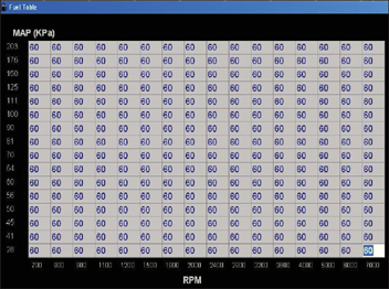
If you’re building a VE table from scratch you have to start somewhere. A constant value is set just to get the engine running long enough to gather some data at part throttle and make some calculated corrections.
With an automatic, it can be a little trickier to control. Below the stall speed of the torque converter, you have a variable slip rate that can make engine speed difficult for the dynamometer to control. If the vehicle is equipped with a lockup torque converter, now would be the time to engage it, once the wheels are moving. Again, third gear usually works well here. If the vehicle does not have a lockup torque converter, steady state high-load test data cannot really be gathered below the stall RPM of the torque converter. Concentrate first on the areas of the map that can be logged in steady state before dropping down to these lower load points. You will often find that adjustments made at a single engine speed can be applied as a percent all the way down to minimum MAP.
The first task is to begin correcting the VE able at a single moderate engine speed. With the dynamometer controls set up to hold a constant speed of approximately 2,000 rpm, use your right foot to maintain a stable load. Also make sure that the engine coolant and air inlet temperatures have stabilized. This is extremely important since aircharge temperature has a significant influence upon calculated airmass. You do not want to perform corrections to the VE table based on varying charge temperatures, so try to keep these temperatures as consistent as possible throughout this exercise. Once both MAP and measured lambda are stable, you are ready to take a valid measurement. Take note of any error in delivered lambda. Since your target is lambda=1.00, a displayed ratio of anything else represents the exact correction factor that should be applied to (multiplied by) the existing VE value in the table.
In a perfect world, individual measurements would be taken at each cell in the VE table. This can prove very time consuming, only to get an initial string of test data that all indicate very similar errors or follow the same trends. To improve the speed of this exercise, it’s possible to take the corrections seen in part of the VE table and apply them to others. Starting at 2,000 rpm and a moderate load of 60 kPa or so, global changes can be made as before in the initial checkout. Moving up in load to perhaps 70 kPa, the changes applied in the 2,000 rpm column can also be applied as a percentage to all speeds at the same 70 kPa load and above. This makes the assumption that if the engine’s pumping efficiency is slightly better (or worse) at 70 kPa, it will continue to be better (or worse) as manifold pressure is increased. Again at 80 kPa, the correction is applied to all speeds at loads of 80 kPa and above. This process can be repeated going downward in measured MAP as well, where corrections found at 50 kPa are applied across all speeds for loads of 50 kPa and below. Again at 40 kPa (if possible, depending on your camshaft selection) the changes are carried downward across all engine speeds as a percentage.

Knowing what fuel is in the tank is critical before diving into the ECU calibration. If you’re buying racing fuel, it’s a good idea to check with your supplier to find out the fuel properties before tuning to an incorrectly assumed stoichiometric air/fuel ratio.
Even at this moderate speed, you may not be able to go all the way up to 100 kPa load on the engine in steady state without fear of knock or high temperatures. Don’t worry, we’ll come back to this later after filling in more of the VE table. For the time being, just go as high as you are comfortable taking the engine with a stoichiometric mixture in steady state.
If, at any point during the volumetric efficiency mapping, spark knock is heard, it must be addressed. Do not continue to operate at a knocking condition for extended periods as engine damage may result. Whenever knock is detected during this exercise, return to the spark advance table and remove timing locally until no further knock is present. Mild knock may only take 2 to 3 degrees to remedy, but don’t be afraid to take more for the time being. You can always add it back in later, after the fueling is dialed-in.
By applying the percent changes seen near 2,000 rpm across all speeds for the same load, the general trend of the engine’s pumping efficiency is more quickly established. After the first corrections are applied at 2,000 rpm, it’s time to move to another speed. Next up should be a slightly higher speed of perhaps 2,400 rpm or so. Your breakpoints don’t have to be exactly 2,000 and 2,400 rpm, just consider these examples for the time being. Even if you started with a completely flat VE table before making the corrections at 2,000 rpm, you should now have some form of linear or curved trend for VE against MAP. The only thing that has really changed now is valve excitation frequency as a result of engine speed. Depending on the cam and intake combination, you may now see slightly higher filling efficiency at 2,400 rpm than was seen at 2,000 rpm. Begin by once again taking a stable reading of lambda error at a moderate load. Apply this correction to the entire column of 2,400-rpm VE points as well as the rest of the VE table for speeds above 2,400 rpm. After all, if pumping efficiency improved by 8% at 2,400 rpm, it can also be expected to improve somewhat at 2,800, 3,600, and 5,000 rpm too, right? The object here is to minimize the corrections you will need to apply later when you finally get to these higher speeds. Then the engine will follow trends and this is one of them. Reducing the time spent at high speeds during calibration also reduces wear on the engine and heat buildup.

Setting a constant target of lambda=1.00 (14.6:1 for gasoline) makes the math easier as you begin calculating individual corrections in the VE table cells. A stoichiometric target means that the instantaneous lambda equals the current correction factor and greatly speeds up the calibration process at part load.

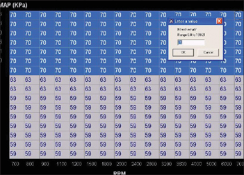
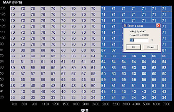
If the engine stabilizes to a delivered lambda of 0.98, this value is used as the correction factor for the entire table for this first adjustment. Multiplying the previous volumetric efficiency value of 60 by the 0.98 correction factor rounds to a new table value of 59 that is used everywhere initially.
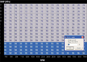
Again at a higher load value another measurement is taken showing a delivered lambda=1.11 at 90 kPa. This 11% increase over the previous value of 63 rounds to an even 70 at this load; and it’s applied across all RPM breakpoints.
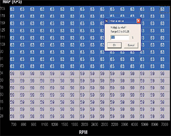
Moving to a higher load/kPa value, the delivered lambda was noted to be about 1.07 in steady state. A 107% correction is then made to all speeds and loads ≥ 70 kPa, resulting in a new value of 63% VE.
Dropping throttle position to a lower load, we see that delivered lambda went rich to an indicated lambda=0.93, so an appropriate correction is made to all low load values. We are now beginning to see the effect of throttle angle and MAP on engine pumping efficiency.
After the moderate load correction for 2,400 rpm is found and applied to everything from 2,400 rpm up, you can get more specific. Increase load again by applying throttle angle and check for error at slightly higher loads. Remember that these corrections should be applied to the “corner” of the table bounded by 2,400 rpm and the current load. Increases or decreases can be applied to this entire corner of the VE table as a percent. This process is repeated for increasing load points at the same 2,400 rpm for an incrementally smaller “corner” of the VE table with each change. You will find that the earlier horizontal scaling found at 2,000 rpm has left you with less work to do here as load is increased at 2,400 rpm. The changes being applied for each smaller size “corner” of the table become smaller as you go. This is further evidence that we’re getting closer to the proper VE surface shape and values as the tuning process continues. If possible, continue this process at 2,400 rpm to as high of a load as you are comfortable running near the nominal temperatures. The same holds true for decreasing loads below our starting point at 2,400 rpm. If you began measurements at 2,400 rpm at 60 kPa, you can now slowly back off the throttle to decrease load to begin mapping the bottom “corner” of the VE table. The same percent-based changes can be applied to the entire corner as you work.
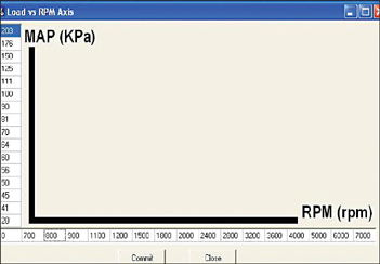
Linear MAP-MAF relationship
This first exercise is generating the fundamental relationship between MAP and airmass for a constant engine speed and temperature. If the VE and airmass (MAF) are plotted against MAP for a single engine speed, we can see an interesting relationship. Figure 10-1 shows this relationship for a sample engine. Notice that there is a straight-line relationship between VE and MAP over much of the measured MAP range. This is not an accident. At a given frequency of valve opening (engine speed), the intake port acts as a fixed pipe that simply flows more or less air in direct proportion to the pressure differential across it. One end is the cylinder at a predictable low pressure and the other is attached to the intake manifold plenum where pressure is measured by the MAP sensor. It stands to reason that the harder the intake manifold pressure is pushing upon the air column in the port, the more flow is realized to the cylinder at the other end. Certainly port tuning has an influence on this, but that is largely tied to intake runner length, volume, and excitation timing of the intake valve from the camshaft. Runner length and volume are fixed, but intake valve event timing is tied to engine speed. So for a single speed point, the relationship between manifold pressure and cylinder filling becomes much more predictable.
In engine calibration, one can use the predictable MAP-MAF relationship to help speed up the process of calibrating the VE table. Not every point along the straight line needs to be collected. We only really need to define the slope of the line and the bounds along which it exists. Points in the middle of the straight line can be interpolated fairly accurately. Below this, it is important to describe the non-linear behavior under high vacuum in order to better estimate aircharge at low loads. Some OEM speed density systems actually use the linear correlation exclusively for airmass estimation. Chances are that if the theory works well enough for these systems to pass the stringent emissions requirements today, they can be applied to the average street rod or racecar with some measure of success.
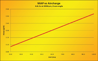
Fig. 10-1 The Ford EFI controllers use a linear MAF estimation based on a simple slope and offset from MAP equation at each RPM breakpoint for backup calculations. The result of these variables at 3,000 rpm and zero cam retard for a 4.6L 3v engine are seen here.
A properly tuned VE table will almost always show this linear relationship as VE values increase predictably with MAP. Common sense tells us that if the manifold pressure is increasing, the cylinder filling should also increase. Unfortunately, some less-experienced tuners miss this key concept and generate VE tables that have spots where VE is either constant or actually decreasing as MAP values increase at the same engine speed. The fundamental cause of this is usually sloppy data collection, but a common sense check should alert the tuner to the fact that this is not probable. Using the linear estimation will prevent the “roller coaster” volumetric efficiency plots that are commonly seen from less-experienced tuners.
Now that engine VE has been mapped at a couple different speeds in the midrange, we begin to see the general trend to the pumping efficiency of this particular hardware combination. Next up is yet another higher speed point, perhaps around 2,800 or 3,000 rpm. The same process is repeated here, starting from a moderate load point of maybe 60 to 70 kPa. Again, the entire column of load points at this speed can be quickly adjusted based on delivered lambda for this first point. Slowly work cell by cell upward in load, making corrections to the upper “corner” of the table as you go. Remember that you don’t have to go all the way to 100 kPa just yet if you aren’t comfortable with it. You can do that later. After the upper “corner” has been adjusted, repeat the process for the lower load “corner.”
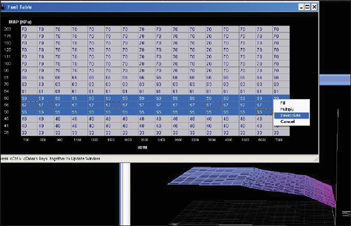
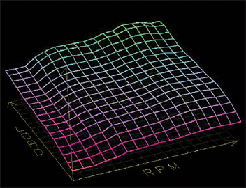
Using the software’s interpolate function, it’s easy to fill in the cells between the first sets of corrections. The 3D map viewed from the side now shows the charateristic quasi-linear increase in volumetric efficiency with MAP. (The flat boosted region has not yet been extrapolated or directly calibrated yet.)
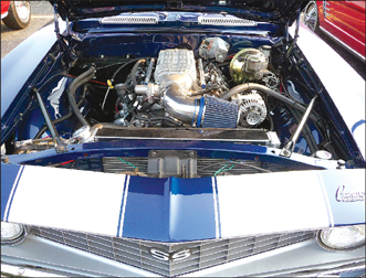
The best of both worlds, gorgeous 1960s sheetmetal surrounding a modern, powerful fuel injected powerplant. The engine in this Camaro spent some quality time on the dyno dialing-in the ECU calibration before being installed so the owner only has to worry about adding gas and driving now.
Notice that at the higher engine speeds, heat builds quickly in both engine coolant and air charge temperature. Keep a careful eye upon both of these as you work to avoid potential damage to components as well as changing air density during this reference work. It’s better to back off for a minute or two and allow the radiator and dyno fans to work than to continue mapping pumping efficiency against changing air density. You want to minimize the variables during the testing process and charge temperature is a big one. The faster the engine speed, the more serious of a concern this becomes. At higher engine speeds, above 3,000 rpm or so, most automotive cooling systems will be seriously taxed by steady state chassis dyno work. Slowly collecting good data here is far more rewarding than quickly collecting questionable data.
Ideally, the high-speed VE mapping is continued all the way to redline. In practice this isn’t always possible due to temperature concerns. This is why the “corner” correction method is so effective. The corner method takes what we have learned at lower speeds and applies the trend to higher speeds. Since the engine is a mechanical pump, it can be expected that its efficiency follows some sort of predictable trend. Even if we can’t collect data at every single point, we can at least extrapolate to get a good anticipation of what the data will probably look like. Generally speaking, you will find that the VE values will increase with speed all the way to the RPM where the engine makes peak torque. Beyond that speed, you will see that VE gradually rolls off with increasing speed. Keep this in mind as you work on mapping the higher speed points of the table.

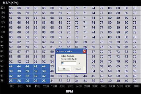
After dialing in the 2,000 rpm behavior, engine speed is allowed to increase to 2,400 rpm on the dyno and a new initial lambda measurement is taken at 60 kPa. A steady state reading of lambda=1.03 is used to correct all values ≥ 2,400 rpm in this example.
Once the higher speeds have been mapped sufficiently, we can begin working back down toward idle. We may not be able to go all the way down to our target idle speed just yet since the lowest point we’ve done is only 2,000 rpm. Below this speed, we may find that volumetric efficiency drops in a nonlinear fashion with respect to speed.
Let’s begin by checking a speed only slightly below our first exercise, perhaps 1,600 rpm. With the vehicle locked into gear and the dyno set to control speed, watch the delivered lambda at a moderate load once again. The delivered lambda error at this moderate load is at first applied to the entire side of the VE table bounded by 1,600 rpm. The final VE values at this lower speed will almost certainly be lower than those at 2,000 rpm because the engine’s pumping efficiency generally decreases at lower speeds. After an initial adjustment based on error at moderate load, we can once again begin working on the “corners” of the VE table as load is increased at lower speeds. The dyno will be responsible for keeping the engine speed in check as load is increased. You will find that the general trend of increasing VE with higher MAP is similar at 1,600 rpm to what was seen at 2,000 rpm, with only slight changes percentage wise. The major difference was the speed change that was accounted for in the first measurement at 1,600 rpm. Work toward increasingly higher loads at 1,600 rpm to check each cell for accuracy being careful to listen for spark knock. It’s surprisingly easy to get knock during these lugging conditions if you aren’t careful. After the high load “corner” is calibrated, move down to the lower load “corner” and repeat the process.
Again at the higher speed, load is increased and another steady state lambda measurement is taken. The new reading of lambda=0.98 is applied as a correction to the remaining “corner” of the VE table.
The lower “corner” of the VE table is corrected based on delivered steady state lambda at 2,400 rpm and 50 kPa. Here, a value of lambda=1.02 is used for all speeds ≥ 2,400 rpm and loads ≤ 50 kPa.
There’s a lot of repetition here, but that’s the nature of calibrating a VE table. A standard 16×16 table has 256 cells in it, and you can expect to perform this process to at least half of them in many cases. Stick with it, because the more precise you are in mapping the VE table, the less work you’ll have to do later when it comes time to address transient fueling and drivability.
Another 2% increase is needed at 2,800 rpm based on a steady state measurement at 70 kPa. The process is repeated to increasing engine speeds as long as the cooling system is able to keep up.

At lower engine speeds, the reduced pumping efficiency is shown as a slightly rich condition before corrections. Here, a reading of lambda =0.98 drives a 2% reduction in the VE values for 1,800 rpm and below.
As you complete the process of mapping the volumetric efficiency of the engine at progressively slower speeds, you will see that there is less and less error in the delivered lambda. By the time you get down to 1,000 rpm or so, you should be pretty close to the target air/fuel ratio. This means that when you actually get to idle speed, you are no longer fighting uncontrolled air/fuel ratio problems such as a lean roll or plug fouling from excessive richness. Even better, the ECU now has a pretty good estimate of actual airmass from which to pull the desired idle air control motor flow. Continue the VE mapping to as low of a stable engine speed as possible. Even if the final target idle speed is going to be 800 rpm, it helps to map the VE table about 100 to 200 rpm lower. This will allow the ECU to accurately calculate airmass whenever engine speed is pulled below idle due to clutch lugging or engagement of accessories like the air conditioning compressor or power steering pump at idle. Later on, when we work on the finer points of idle control we can at least say with confidence that airmass estimation and air/fuel ratio control are not the problem.
After mapping the majority of the VE table, we have learned quite a bit about the engine’s characteristics. Even though we haven’t yet taken this engine to WOT, a good estimate of the expected performance can be made. By following the linear MAP-MAF trend discussed earlier, VE values at 100 kPa can be extrapolated from the part throttle values in the accompanying sidebar at each speed breakpoint. Simply follow this linear trend upward to populate the 100 kPa line and blend smoothly between there and the lower points that were more precisely measured earlier.
Working to progressively lower engine speeds and loads gets you closer to the idle region. By the time you actually reach the idle cells, the values will end up being very close and the engine is less likely to stall or load up due to fueling issues.
With a naturally aspirated engine, you are now ready to prepare for the first WOT test on the dyno. If you are testing a supercharged engine, the first test will only target 100 kPa load. This can be accomplished by either careful modulation of the throttle to avoid boost, or by removing the supercharger drive belt if possible. Turbocharged applications will likely need to stick to careful throttle modulation since some boost creep is usually present even with a fully open wastegate. Since the object is to only run the equivalent of a naturally aspirated engine’s performance, a target ratio of lambda≈0.85 can be used for all applications at this load. Set the same target ratio for all engine speeds and all loads from about 90 kPa to 105 kPa. This will help ensure that you are not chasing a moving target for air/fuel ratio when recording.
Make sure that the ignition timing is set very conservatively. You don’t want to experience potentially dangerous knock just because the initial VE estimation was slightly low. The purpose here is to solve for proper VE estimation based on measured lambda, not to make the big power number just yet.
Start the run from a relatively low speed, perhaps 1,500 rpm or so in third or fourth gear. Engine dynamometers can be set to a sweep rate of approximately 300 rpm/sec to match what is typically seen on the road under load. Perform the first WOT run with datalogging active to record delivered lambda, MAP, and engine speed. Continue the run as high as possible unless either knock or an excessively lean air/fuel ratio requires you to stop. Go back through the recorded data to compare the delivered lambda to the commanded reference at each table breakpoint. For example, a delivered lambda of 0.91 at one point would require a correction factor of (0.91/0.85) = 1.07 to bring fueling into line. In this case, we saw a delivered air/fuel ratio that was 7% leaner than commanded so the corresponding volumetric efficiency is increased by that same 7% locally to increase the airmass calculation. If the fuel injector characterization was right, the ECU will automatically add 7% more fuel the next time around to go along with the 7% greater airmass calculation. This process is repeated at each breakpoint until the delivered lambda matched the commanded lambda at all speeds up to redline. Even if the spark advance isn’t completely optimized, the engine should still show decent power. This will be fine tuned later.
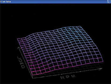
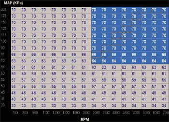
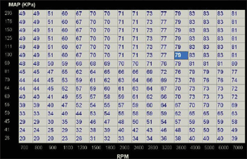
Here’s the result of the VE table corrections using the “corner” method for all part-load conditions. Viewed in 3D, the table is smooth and progressive, just like the engine’s actual pumping efficiency.
The concept of the linear MAF-MAP relationship is not limited to the vacuum region of engine operation. The boosted region can also be approximated by a straight-line extension of the lower load region, at least as a starting point. If starting from scratch on a supercharged or turbocharged engine calibration, using an extrapolation of the low load data to populate the boosted region’s VE values can be a handy tool to reduce overall time spent on the process.
The approximation is started by examining the slope of the VE values at a single engine speed. The slope is found by finding the rise (change in VE) over the run (change in MAP) for the speed column in question. This gives us the following formula:

For a pair of points of 0.735 VE at 72 kPa and 0.877 VE at 101 kPa, the slope is calculated as:

This calculated slope of about 0.5% VE increase per kPa of manifold pressure can be used to solve for a new maximum boost volumetric efficiency estimate. If the engine is set up to make an additional 10 psi (69 kPa) of boost beyond atmospheric levels, then we use this slope to calculate how much higher the volumetric efficiency might go. In our example here, we calculate the increase in VE as:
VE increase = (0.0049 VE / kPa) × (69 kPa) ≈ 0.338 VE
This increase is over and above the volumetric efficiency of the engine at 101 kPa as seen earlier. If we add this theoretical increase of 0.338 to the calculated value of 0.877, we come up with an estimated 1.215 volumetric efficiency. This may not be the actual pumping efficiency seen by the engine at 10 psi of boost for our speed in question, but it gives us a good starting point before we take the engine into uncharted territory under load. Once a single point relatively high in the boosted region has been calculated, most ECUs will have an interpolate function that will fill the cells in between with a straight-line calculation, another real time saver. It may be helpful to set up a quick Excel spreadsheet to calculate the slope at each individual speed breakpoint.
It’s better to overestimate the boosted region VE values at first to avoid knock or excess temperatures that may lead to engine damage. You can always lean it out later if the testing shows that this estimate was too rich, even for the safe boosted target ratio. This linear extrapolation is intended to quickly fill in an area of the VE table that can be difficult to reach and has the potential for some expensive damage if done wrong. In the end, the ideal calibration values will be found based on the usual testing where lambda errors are examined on a cell by cell basis within the VE table.
With the engine’s volumetric efficiency properly mapped up to and including atmospheric conditions, boosted operation is next. The lessons learned at lower loads are applied to the boosted region just as they were at 100 kPa. An extrapolation of the linear trend can be applied well into boost. In reality, this will work fairly well at moderate boost levels and most likely overestimate pumping efficiency slightly at elevated boost levels. There are diminishing returns of airmass increase with manifold pressure increases.
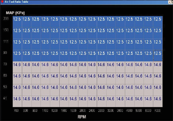
Before running the WOT test, it’s important to choose a new target air/fuel ratio. A value of lambda=0.85 (12.5:1 gasoline) should be a safe target for naturally aspirated engines or boosted engines operating at 100 kPa.
In an ideal environment, each boosted cell in the VE table would be mapped in steady state just as with the vacuum cells. An engine dyno can make this task exceptionally more precise as long as proper cooling capacity is available. Steady state boosted testing really isn’t practical with engines installed in the vehicle, since the cooling systems are rarely up to the task. In this case, it is advisable to slowly work upward through the MAP rows by performing WOT sweep tests at progressively higher pressures. After each sweep test, corrections are made to individual points based on delivered lambda error. Any significant changes are also extrapolated upward to higher pressures at the same engine speed to minimize the error on each following WOT sweep. The process is continued until maximum desired boost is reached and all points are able to deliver the commanded air/fuel ratio.
During the WOT testing at atmospheric levels, the recorded data should be analyzed on a cell-by-cell basis along the 100 kPa line (at sea level). Individual corr-ections can be made to a single cell at a time based on instantaneous lambda error.
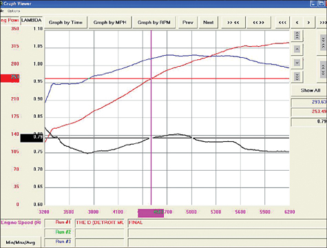
After the WOT dyno run has been performed, the recorded dyno data can be reviewed in detail. This run showed a delivered lambda=0.792 at 4,500 rpm, which will be used to calculate the necessary VE correction factor based on the target lambda.

Operating in the boosted region requires some additional fueling to aid in cooling and knock control. A constant target ratio of lambda=0.78 (11.5:1 gasoline) is a good starting point just in case the initial tests are slightly leaner than the target before corrections.
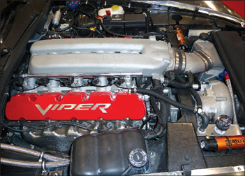
Don’t be intimidated by the huge power potential of this 8.3 L supercharged V10. Tuning this car is just like any other. Start in the midrange and slowly work your way into the boosted region to unlock the power.
When VE mapping is complete, the result should be a very smooth and progressive map. When viewed in three dimensions, it should not show any “mountains” or “canyons” in the middle. Engines are mechanical pumps that do not want to have drastic changes with either speed or pressure. As such, their efficiency maps will be smooth with some “island” of peak efficiency in the middle. This efficiency island will match with the engine’s torque peak since cylinder filling closely approximates potential energy of the charge. The points at which more charge is loaded into the cylinder represent more potential cylinder pressure and torque output on the power stroke. Naturally, any point where the ram tuning of the intake, camshaft, and exhaust system enhance the engine’s pumping efficiency will show up as larger local values in the VE map.
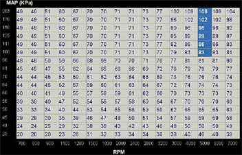
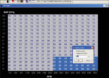
Extrapolating the slope of the VE versus MAP from the lower load region into the boosted region gives the calibration an excellent starting point. In this case, a slope of 0.25% VE per kPa is found between 60 and 100 kPa at 5,000 rpm and used to populate the table all the way up to 203 kPa.
With the boosted region now updated, we get a better look at the engine’s complete VE surface. Notice how even the high load region is still smooth and progressive.