One key skill in working with data is the ability to separate, rearrange, and group a data set in different ways. Sorting and filtering can get you a long way.
The following sections describe some helpful uses of sorting. But before we dive in, let’s go over some important rules you need to follow to get Excel to cooperate with you. These sorting rules really get into the fundamentals of good spreadsheet development because they not only apply to sorting but also Pivot Tables, VBA coding, and other features of Excel that can make your work easier.
The Data Range Must Be Contiguous (No Completely Blank Rows or Columns)
In this figure, if you sorted by column B with the data set as it is—that is, with column C empty—only columns A and B would be included in the sort:

What if you’re in a situation where someone insists that there be an empty column C? One way to make the data contiguous is to place a character, any character, in column C and color it white. Excel will read the data set as one solid range—even though the data set will still appear to be separated—and sort it all.
|
Sometimes people use blank columns to make small gaps between the columns, as shown in the next figure. They simply want the column heads to have some space between them. |
|


TIP
The flip side is that you can intentionally include blank rows or columns in order to confine sorting to a particular part of the sheet. For example, when you have unrelated data in a single worksheet, you may want to use a blank row or blank column to ensure that sorting doesn’t impact all the unrelated data.
Headings Must Be Only One Cell Tall
In the figure below, Favorite will be treated like a heading, and the items in row 2 (Name, Color, and Activities) will be sorted with all the data from the rows below.

Sometimes you need the data in a cell to be on more than one line, but you also need the data to stay in just one cell. There are two solutions to this dilemma:
- Wrap text. (As shown in the figure below)
- Place your cursor between the words that need to be split and then press Alt+Enter. That starts a new line for everything after the cursor.

The following figure shows a merged cells error.

Adding shading to the cells reveals the problem. You can now see that cells C4 and D4 are merged:

TIP
Sometimes you might have a particular spreadsheet in which the merged cells warning keeps popping up, preventing you from getting any work done. Merged cells are hard to find, and that merged-cell error is annoying because you don’t know if there are no more merged cells or thousands more, so here’s another way to deal with this:
Select the entire worksheet by clicking the box above and to the left of cell A1.
Open the Format Cells dialog by pressing Ctrl+1.
On the Alignment tab, you will see that Merged Cells is neither checked nor unchecked. The blue fill indicates that some cells are merged and others are not. Click the Merged Cells checkbox twice. The first will change to checked. The second click will clear all merged cells. This type of checkbox is called a Tri-State checkbox. When it is in the "mixed" state, click twice to turn off that property in all cells.
CAUTION
There are many reasons why merged cells are evil and should be avoided. If you are selecting cells by dragging the mouse or using Shift+Arrow Keys, Excel will make your selection as wide as the merged cells if you accidentally touch the merged area.
NOTE
If you were using Merged Cells to nicely center a heading, the Center Across Selection will give you the same result without the evilness of Merged Cells. Select the range where the heading should appear, then use Format Cells | Alignment | Horizontal | Center Across Selection.
As shown in the next figures, the three sorting options are in the Data tab of the ribbon, in the Sort & Filter group.
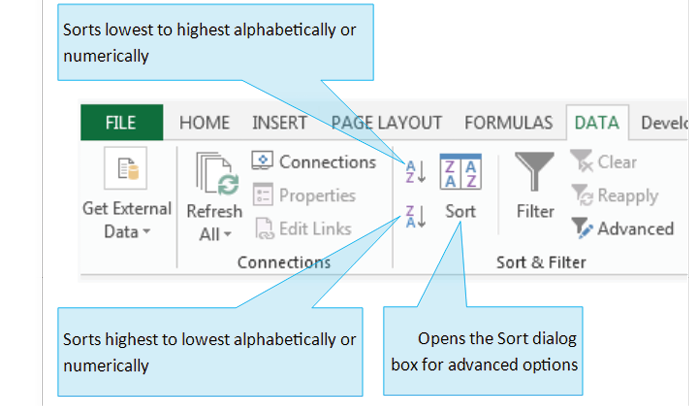
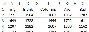
To use the quick-sort icons (the ones with AZ or ZA and the down arrow), you simply place your cursor in a single cell in the data range, in the column that you want to sort by. Excel sorts the column as soon as you click the icon. It’s important that you make sure everything is set up properly before you click the icon. If your columns have headers, you need to be sure that they are somehow distinguishable (with bold or all caps, for instance). Otherwise, Excel will assume that you have no headers and will sort the entire column, with the headers mixed in with the content.
|
In this figure, Excel sorted three columns, starting with Colors as the heading. Excel sorted columns F and J accurately. Column H, though, has a problem: Excel saw its heading, Colors, as another entry in the list and alphabetized it as if it were a regular entry. In this case, the bold applied to F1 and the all caps applied to J1 were enough to have Excel determine that these were headings. |
|

Understanding Ascending and Descending Sorts
When you click the ascending sort icon with text selected, Excel sorts the list alphabetically or numerically, starting at the beginning of the alphabet or the smallest number. When you click the descending sort icon, Excel goes the other way, sorting from Z to A or from the largest number to the smallest. Excel knows only alphabetical order with text sorts. If you want to sort by a date presented in text form or another value that has a known order, the sort feature will not respect that. For example, an ascending sort for days of the week will normally result in this order:
Friday, Monday, Saturday, Sunday, Thursday, Tuesday, Wednesday
To have the days of the week instead sort into the chronological order people expect, open the Order dropdown and choose Custom List, as shown here:

Then, in the Custom Lists box, shown below, select Sunday, Monday, Tuesday,....

NOTE
Say that you have to sort a data set with PTC-710, PTC-960, and PTC-1100. An alphabetical sort would always put PTC-1100 before PTC-710. To solve the problem, you can type the list in the proper sequence and then select File | Options | Advanced. On the Advanced tab, scroll all the way to the bottom and choose Edit Custom Lists. Then select the cells with the proper sequence and import this as a new custom list. You can then use that list for sorting the products into the proper sequence.
A custom list can contain from 2 to 180 items. Each item can be up to 255 characters.
Let’s Get Some Data Sorted Out
Now it’s time for you to try some sorting. The following figure shows 49 rows of data, representing website activity by country/territory.

Say that you want to sort this data so it’s sorted from highest Pages/Session value to lowest.
With the cursor in column G of the data set, select the descending sort icon (ZA). You get this result:

You can see that Taiwan is at the top of the list, with 3.69 pages per session. You can also see that the number of sessions for Taiwan is 42, and the number for Malaysia is 205. Your analyst sense tells you that maybe there isn’t a story in the Taiwan data, but there’s something in the Malaysia data.
Now say that you’re only interested in entries where the Sessions value is greater than 100. To visually set apart the countries/territories with more than 100 sessions from those that have 100 or fewer, you could do a descending sort in the Sessions column and insert a blank row between more than 100 sessions and 100 or fewer—in this case, between Romania and Greece:

Now when you work with the data above row 32, you will be working with data that seems to have a significant amount of information to work with.
NOTE
Before you move on to the next section, delete the empty row you just inserted so that you’re working with the full data set.
To continue exploring sorting, let’s look at the same data as in the last section, this time sorting by region and then by country.
To sort by these two criteria, follow these steps:
1.Put your cursor in any column or row of the data range.
2.Click the large Sort icon. The Sort window appears:

3.Click Add Level to sort by two criteria.
4.Ensure that the My Data Has Headers check box is selected.
5.For the first sort, set Sort By to Region, Sort On to Values, and Order to A to Z.
6.For the second sort, set Then By to Country/Territory, Sort On to Values, and Order to A to Z.
7.Click OK.
|
Excel performs the sort, and the regions are now grouped together alphabetically, as you can see in the next figure. Then the countries are shown in alphabetical order, listed alphabetically within the regions. TIP The sorting options are very helpful, so you should do some exploring. You can even sort horizontally, not just vertically. Dig in there and get some ideas about what’s possible. |
|

Sorting with the Help of a Helper Column
Sometimes sorting alone isn’t enough to find the information you want, and you have to be extra clever. Say that you have 50 employees who need to complete three training programs, and you want a list of who has not completed them (see the next figure). This means you need to find a way to group the people who’ve completed three trainings and separate them from the people who’ve completed zero, one, or two trainings. Sorting alone won’t handle this for you, but with some figuring, you can make it happen.
