2
Structure of Turbulent Boundary Layers
ABSTRACT
The coherent eddy structures that have been discovered to date are reviewed and discussed. These include the near-wall low speed streaks and quasi-streamwise vortices, hairpin vortices and hairpin vortex packets, large-scale motions and very large-scale motions. Interactions between the different scales are discussed and the experimental problems of observing coherent structures in geophysical flows are considered.
2.1 Introduction
Turbulent boundary layers and related flows, in the canonical geometries of pipes, channels and open channels, share many common characteristics. The effect of viscosity is confined mainly to a thin region above the wall called the buffer layer, the mean velocity varies logarithmically between the buffer layer and a few tenths of the flow depth, and a region of wake-like behaviour occupies the remainder of the flow. The kinematic viscosity  , the wall shear stress
  and the outer length scale
  (either boundary layer thickness δ, pipe radius R, or channel depth h) are the essential parameters of these flows, and the appropriate nondimensional form of the distance above the wall y is
  in the inner layer, consisting of the buffer layer plus the logarithmic layer, and
  in the outer layer, consisting of the logarithmic layer plus the wake layer. Here,
  is the friction velocity and ρ is the fluid density. The buffer layer extends up to y+ = 30, conventionally; the logarithmic layer extends from the top of the buffer layer to
  , and the wake region extends from the top of the log layer to the full layer depth. The von Kármán number, defined as the ratio of the outer length scale to the viscous length scale, is equal to the Reynolds number:
It is a convenient nominal measure of the range of eddy sizes. Clearly geophysical flows, which have very large Reynolds numbers, contain eddies whose sizes vary over an enormous range.
The foregoing definitions are based entirely on the behaviour of the mean velocity profile, which, for many years, was the main source of information about turbulent flow behaviour. More recently, Wei et al. (2005) identified a four-layer structure based on the changing balance of the terms in the mean momentum equation governing the mean velocity U. (The fluctuating velocity components in the streamwise, wall-normal and spanwise directions will be denoted by u, v, w, respectively, and position coordinates are x, y, z.) These terms consist of the mean advective acceleration for boundary layers, or the mean pressure gradient divided by density for pipe and channel flow or the streamwise component of gravitational acceleration for open channel flow balanced by the gradient of the viscous stress,  and the gradient of the Reynolds shear stress,
  , also called the net force. In the inner viscous sublayer, viscous force balances convection, pressure gradient or gravity from the wall to y+ = 3. In the stress gradient balance layer between
  viscous force balances the net Reynolds force. This layer is much like the conventional buffer layer except for the limit of its upper extent. Interestingly, viscosity plays a further role above this layer because the gradient of the Reynolds stress vanishes at approximately
(2.2) 
the empirical location of the maximum Reynolds shear stress. Therefore, the mean viscous force is needed to balance the mean convection or pressure gradient or gravity at and around this location, as in the inner viscous sublayer (Sreenivasan, 1989). Above y+p the net force represented by the gradient of the Reynolds shear stress decelerates the mean flow, and below it the net force is accelerative. The range in which the viscous force balances the advection or the pressure gradient or the gravitational force is  (Wei et al., 2005). It is referred to as the mesolayer. Above it, the gradient of the net Reynolds stress balances the advection or the pressure gradient or the gravitational force, and the length scale becomes
  . The mean velocity varies logarithmically up to
  , and then transitions into wake-like behaviour. According to Equation (2.1),
  becomes a vanishing fraction of the layer depth
  in the limit of infinite Reynolds number.
The boundaries of geophysical flows are very often rough, causing the layers near the wall to be disrupted. Even so, above the layer influenced by roughness, the logarithmic layer persists with substantially the same von Kármán constant, but an additive constant is needed to represent the velocity at the top of the roughness elements. This behaviour implies that the layers near the wall are not essential to the formation of the eddies that characterize the logarithmic layer.
2.2 Eddy structures
The study of coherent eddies in turbulent flow is an attempt to reduce the complexity of random three-dimensional turbulent motions to a collection of simpler motions that can be classified according to shared characteristics of their flow patterns. Eddies usually possess vorticity in a compact region and persist for a period long enough to make significant contributions to the time averaged statistics of the flow. In this sense, they are coherent structures or organized motions (Marusic and Adrian, 2012).
2.2.1 Near-wall quasi-streamwise vortices
Above a smooth wall, the buffer layer contains high-speed and low-speed streaks of fluid whose mean spacing, in viscous wall units, is  at the wall. (The more commonly quoted value of
  pertains to the mid-point of the buffer layer.) The streaks are caused by quasi-streamwise vortices, (long, thin tubes of vorticity that are oriented mainly in the streamwise direction, Figure 2.1a) whose diameters are about 40+, corresponding to 22 Kolmogorov length scales. The vortices occur in counter-rotating pairs such that, in the region between the pair, a left clockwise and right counterclockwise pair induces flow downward toward the wall, and a left counterclockwise-right clockwise pair moves fluid upward away from the wall. The downflows carry high momentum fluid and create high-velocity streaks, and vice versa for the upflows. The correlations between the velocities in downflows v < 0, with positive streamwise fluctuations, u > 0 and upflows v>0, with negative streamwise fluctuations, u < 0 produce the net positive mean Reynolds' shear stress,
  .
.
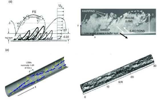
Figure 2.1 Coherent structures of wall turbulence. Idealized depictions are presented in the left column for clarity, and sample realizations are presented in the right column. (a) Low speed streaks in the buffer layer. Regions of up flow +v and down flow –v are associated with low speed fluctuations –u and high speed fluctuations +u; (b) First generation hairpin vortex generated above the buffer layer; (c) Hierarchy of hairpin vortex packets convecting at velocities Uc1 < Uc2 < Uc3; (d) Large scale motions (LSM) or turbulent bulges formed at the edge of the turbulent layer. I and II denote first and second generation packets, U0 is the free stream velocity and δ is the boundary layer thickness; (e) Very large scale motions (VLSM) in pipe flow. R is the pipe radius. In all panels streamwise, vertical and spanwise directions are x, y and z, respectively. Reprinted from Zhou et al., 1999, with permission from Cambridge University Press. (c left) Reprinted from Adrian, et al., 2000, with permission from Cambridge University Press. (c right) After Hommema and Adrian, 2003. With kind permission from Springer Science and Business Media. (d left) Reprinted with permission from Adrian, 2007. Copyright 2007, American Institute of Physics. (e left) Reprinted from Baltzer et al., 2013, with permission from Cambridge University Press. (e right) Reprinted from Wu et al., 2012, with permission from Cambridge University Press.
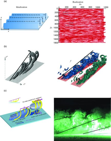
Eddies take various forms throughout the boundary layer, but in all cases the upward transport of low streamwise momentum and the downward transport of high steam wise momentum is the fundamental mechanism responsible for the creation of Reynolds shear stress. This is very much like the arguments in classical mixing length theory, except that the eddies are allowed to have varying orientations and shapes.
2.2.2 Hairpins and hairpin vortex packets
In the log-layer, the main eddy shape is that of a hairpin with legs emerging from the quasi-streamwise vortices (Figure 2.1b). This is an average shape that is necessarily symmetric with respect to the x–y plane. Instantaneously, the shapes are almost always asymmetric, with one leg stronger than the other, looking like canes, rather than hairpins. The term turbines propensii has been suggested to encompass the full class of inclined vortices and avoid implying that the geometry of the eddies is too specific (Marusic and Adrian, 2012). The turbines propensii constitute the attached wall vortices in the sense of Townsend (1976). If a hairpin emerges from the buffer layer with sufficient rotational strength, it can create secondary hairpins upstream and downstream of the parent, a process referred to as auto generation of hairpins (Zhou et al., 1996, 1999). Once started, the secondary hairpins can auto generate tertiary hairpins, and so on, leading to a packet of hairpins in which the tallest hairpin is the parent and the smallest hairpin is the most recently born. Auto generation proceeds at roughly equal time intervals, so the hairpins are spaced fairly equally, and packets take the form of ramps (Figure 2.1c). Evidence, mostly from laboratory investigations (Bandyopadhyay, 1980; Head and Bandyopadhyay, 1981; Adrian et al., 2000), indicates that ramp angles lie between 13 and 18°. Using experiments in the atmospheric surface layer, Marusic and Heuer (2007) have demonstrated invariance of this angle over a 1000:1 range of Reynolds numbers with a mean angle of 14.5°.
Early direct numerical simulations of the evolution of initially symmetric disturbances predicted symmetric hairpin packets (Zhou et al., 1996). But later simulations starting from slightly asymmetric disturbances predicted much more complex behaviour, with the vortices tangling, cutting, and reconnecting, as in Figure 2.1b (right). Despite this complexity, the packets retain the characteristic ramp shape. Observations in higher Reynolds-number laboratory flows with smooth surfaces reveal the ramp patterns at several levels throughout the boundary layer (Adrian et al., 2000; Carlier and Stanislas, 2005; Ganapathisubramani et al., 2003). They are also observed above rough surfaces (Detert, et al. 2010; Guala, et al., 2012), indicating a robust propensity for the flow to generate ramps, and presumably packets of vortices, even when the viscous buffer layer is destroyed.
A limited number of atmospheric flow experiments (Hommema and Adrian, 2002; Marusic and Heuer, 2007; Morris et al., 2007) confirm the occurrence of packets, and theoretical considerations demonstrate their importance (Marusic, 2001). Because of the scale of atmospheric observations, it is difficult experimentally to visualize the hairpin vortices per se, and proof of their existence is indirect, resting mainly on the ramp shapes and what looks like the heads of hairpins on the edges of the ramps (Figure 2.1c, right). Observations of ramp-like vortex packets at heights greater than 1 m above the ground imply that small, first-generation packets, with typical height of 10–50 mm, somehow grow into much larger packets. The mechanism for this growth is thought to be the merging of packets as they grow into each other. This process can be seen in direct numerical simulation of first-generation packets growing into second generation packets, but it has so far eluded unequivocal experimental observation, in part because larger eddies have weaker vorticity and are harder to visualize.
The linear growth of the packets in the logarithmic layer produces a linearly increasing length scale (Tomkins and Adrian, 2003) that is consistent with the linear variation of the mixing length known from mixing length theory and, indeed, any other scaling theory of the log-layer. The ramp angle is a fundamental characteristic of the linear growth of the hairpins, and constancy of the ramp angle in the log-layer is likely to be involved in theoretical derivation of von Kármán's constant. Packets are not, however, confined to the logarithmic layer. They are observed to sometimes poke well above it, reaching even to the outer edge of the boundary layer, as in the seminal observations of Bandyopadhyay (1980) and Head and Bandyopadhyay (1981).
2.2.3 Large-scale motions
The well-known turbulent bulges (Kovasznay, et al., 1970; Cantwell, 1981) share many similarities with large hairpin packets, and it is possible that they are one and the same (Figure 2.1d). The visualizations of Head and Bandyopadhyay (1981) would certainly suggest so. But better evidence is needed to fully establish the links between bulges and packets. Current practice classifies bulges as large-scale motions (LSM) whose lengths are approximately two-to-three times the boundary layer thickness. Large-scale motions also occur in pipe, channel and, probably, open-channel flows with streamwise lengths of about two-to-three layer depths, but without, of course, the bulge geometry. The evidence for LSMs in these flows comes from frequency power spectra of the streamwise velocity. The large-scale motions persist out to about y/δ ∼ 1, consistent with the bulges observed in visualizations (Balakumar and Adrian, 2007). The departure of the mean velocity profile from the logarithmic law occurs in the region dominated by the bulges, suggesting a close relationship. In particular, the irrotational fluid between the intermittent bulges (see Figure 2.1d) implies a reduction in the average Reynolds shear stress, consistent with the increased mean velocity gradient observed above the logarithmic layer.
2.2.4 Very large-scale motions
Very large-scale motions (VLSM) were discovered in pipe flow from close examination of the spectra of the streamwise velocity (Kim and Adrian, 1999). They are defined as motions longer than two-to-three layer thicknesses, and they can extend more than 15–20 pipe radii in the streamwise direction. Later work in pipe flow (Guala et al., 2006) showed that they extend from the wall to about one-half pipe radius and were strongest in the log layer. Most importantly, they contain substantial fractions of the total turbulent kinetic energy and the Reynolds shear stress, making them essential to consider when modelling turbulence. Recent studies of a direct numerical simulation of a 30R long pipe flow with Reynolds number 24 500 (Wu et al., 2012; Baltzer et al., 2013) show that the very large-scale motions are concatenations of LSMs and smaller motions, as originally conjectured by Kim and Adrian (1999). However, the concatenation occurs along an angle to the pipe axis, and it is associated with spiral roll cells. The roll cells are similar to those inferred from the behaviour of surface motions in open-channel flows. Evidence of large, long, meandering and streamwise-inclined eddies in open channel flows supports the paradigm just described (Adrian and Marusic, 2012).
Very large-scale motions also occur in channel flows (Balakumar and Adrian, 2007) where, as in pipe flow, they account for large fractions of the energy and Reynolds shear stress. In boundary layer flow they are shorter, of the order of 6–7δ, and there is some uncertainty as to whether they are different from the bulges or merely longer than average bulges (Hutchins and Marusic, 2007, Monty et al., 2009). Evidence for VLSMs in the atmospheric surface layer also comes from Hutchins and Marusic (2007), who used arrays of hotwires to infer lengths of 10δ, or more. Support for the concatenation hypothesis of Kim and Adrian (1999) applying to the turbulent boundary layer comes from atmospheric surface layer and laboratory measurements found in Hambleton et al. (2006) and Hutchins et al. (2012).
2.3 Interactions of eddies on different scales
The interaction of the inner scales with the outer scales, or the absence thereof, has been a topic of long debate in the study of wall turbulence. No interaction would imply that the inner layer is free standing and dynamically autonomous, and this would be convenient theoretically. However, recent work from the University of Melbourne (Marusic et al., 2010) clearly shows a dynamic correlation between times series measurements in the two layers in which large-scale motions from the outer layer do two things: (i) they leave an additive imprint, or footprint, on the streamwise velocity field in the near wall region; and (ii) they stimulate small-scale activity in the inner layer during periods of large-scale acceleration. This second effect is manifested as a multiplicative factor.
Physically, the observations of Marusic et al. (2010) are quite reasonable if one views wall turbulence from the viewpoint of boundary layer theory. The large-scale outer flow scales in outer variables, and its velocity at the wall, would provide an upper boundary condition for the inner layer, which scales in viscous wall variables (i.e. + units) and contains the molecular viscosity needed to satisfy no slip at the wall. The upper boundary condition on the inner layer couples the inner and outer motions. Increasing outer flow velocity implies larger inner flow velocities and increased stretching of the small-scale eddies, thereby stimulating them, and it forms a multiplicative scale. That is, doubling the outer flow doubles the inner flow velocities. Physically, we can only observe the composite solution from such a model, which is the sum of the inner and outer solutions minus the common part. The summation is consistent with the results found by Marusic et al. (2010).
The concept of inner/outer interaction stimulates thinking about dynamic processes. For example, a large-scale high-speed region displacing a large-scale, low-speed region would stimulate the small-scale hairpins to greater activity. Their function is to pump low-speed fluid upward into the high-speed region, thereby decelerating it. Lower speed in one locale implies, by continuity, higher speed in another, so a new high-speed region must be formed at a different location, and the process is repeated there. This could lead to a cyclic pattern of high speed and low speed regions in the outer layer.
2.4 Extracting coherent structure from geophysical flows
Geophysical flows offer unique opportunities to study turbulence at very high Reynolds number. They also pose extraordinary challenges owing to inability to control them and the instrumental scale. Thus, while laboratory flows are accessible to high-resolution PIV measurements, geophysical flows are more likely to be studied with lower resolution scanning 3-D radar or LiDAR instruments, making observations of eddies difficult. Higher resolution can be achieved by acoustic Doppler or thermal anemometer probes, but only on a coarse grid of points. The challenge is to find aspects of the turbulent motion that can be measured in both the laboratory and the field. In this regard, the low-momentum zones inside the hairpin vortex packets seem much more likely to be observed than the vortices that surround them, owing to the lower resolution required to see them.
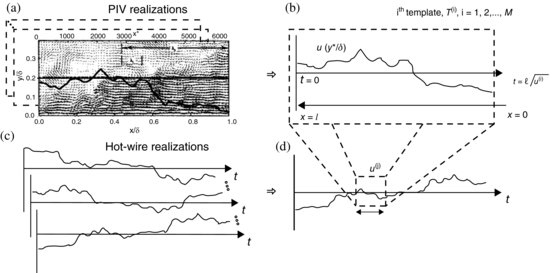
One approach to this problem has been described by Hommema and Adrian (2002), who used a template-matching scheme in which samples of line series data through turbulent ramps from laboratory experiments (Figure 2.2) were matched to segments of time series data from a hot wire probe in the atmosphere. Matching was performed by stretching the laboratory data and translating it along the atmospheric time series, looking for positions of least mean square error. It was found that using only eight of the laboratory templates allowed more than 50% of the atmospheric signal to be reconstructed with 65% correlation coefficient. Moreover, the eight different templates were each passages through vortex packet ramps.
Figure 2.2 Schematic representation of the template-matching procedure. (a) Ensemble of M PIV realizations; (b) A template T(i) is extracted from each of M PIV realizations at a specified vertical coordinate (y/δ); (c) Ensemble of hot-wire realizations; (d) Template is correlated with the moving window, u(j), in each hot-wire record to generate the coefficient gi,j. This procedure is performed for each hotwire realization, generating N correlation coefficients for each template. Reprinted from Hommema and Adrian, 2002. With kind permission of Springer Science and Business Media.
The process was fundamentally the same as the well-known wavelet analysis (Seena and Sung, 2011), except for two extremely important differences. First, it applied only one stretching to the laboratory data, while wavelet transforms systematically vary the dilation parameter. Second, instead of using an ad hoc wavelet kernel such as a Mexican hat, which has no physical relation to the turbulence, the template-matching approach used a set of wavelet kernels taken from the structure of the flow. In actuality, the process started with about 20 templates selected randomly, and determined which parts of the atmospheric signal could be represented by the various templates. The wavelet transform should be exploited for this problem because systematic dilatation permits extracting different scales of eddies.
2.5 Conclusions
Much is known about the coherent eddies of wall turbulence, but an even greater amount remains to be learned. Geophysical flows have great potential to contribute to our knowledge in this area, largely owing to the very large Reynolds numbers that can be accessed in these flows. While the buffer layer plays a big role in low Reynolds number experiments and simulations, it is likely to be irrelevant in geophysical flows, and the most profitable and appropriate focus of the research is likely to be the low momentum zones in packets and the very large-scale motions.
2.6 Acknowledgements
This research was supported by a grant from the US National Science Foundation and the Ira A. Fulton Endowment, Arizona State University.
References
Adrian, R.J. (2007) Hairpin vortex organization in wall turbulence. Physics of Fluids 19, 041301.
Adrian, R.J. and Marusic, I. (2012) Coherent structures in flow over hydraulic engineering surfaces. Journal of Hydraulic Research 50, 451–464.
Adrian, R.J., Meinhart, C.D. and Tomkins, C.D. (2000) Vortex organization in the outer region of the turbulent boundary layer. Journal of Fluid Mechanics 422, 1–53.
Balakumar, B.J. and Adrian, R.J. (2007) Large- and very-large scale motions in channel and boundary layer flows. Royal Society of London Transactions A365, 665–681.
Baltzer, J.R., Wu, X. and Adrian, R.J. (2013) Structural organization of large and very-large scales in turbulent pipe flow simulation. Journal of Fluid Mechanics 720, 236–279.
Bandyopadhyay, P. (1980) Large structure with a characteristic upstream interface in turbulent boundary layers. Physics of Fluids 23, 2326–2327.
Cantwell, B.J. (1981) Organized motion in turbulent flow. Annual Review of Fluid Mechanics 13, 457–515.
Carlier, J. and Stanislas, M. (2005) Experimental study of eddy structures in a turbulent boundary layer using particle image velocimetry. Journal of Fluid Mechanics 535, 143–188.
Detert, M., Nikora, V. and Jirka, G.H. (2010) Synoptic velocity and pressure fields at the water–sediment interface of streambeds. Journal of Fluid Mechanics 660, 55–86.
Ganapathisubramani, B., Longmire, E.K. and Marusic, I. (2003) Characteristics of vortex packets in turbulent boundary layers. Journal of Fluid Mechanics 478, 35–46.
Guala, M., Hommema, S.E. and Adrian, R.J. (2006) Large-scale and very-large-scale motions in turbulent pipe flow. Journal of Fluid Mechanics 554, 521–542.
Guala, M., Tomkins, C.D., Christensen, K.T.C. and Adrian, R.J. (2012) Vortex organization in a turbulent boundary layer overlying sparse roughness elements. Journal of Hydraulic Research 50, 465–481.
Hambleton, W.T., Hutchins, N. and Marusic, I. (2006) Simultaneous orthogonal plane particle image velocimetry measurements in a turbulent boundary layer. Journal of Fluid Mechanics 560, 53–64.
Head, M.R. and Bandyopadhyay, P.R. (1981) New aspects of turbulent structure. Journal of Fluid Mechanics 107, 297–337.
Hommema, S.E. and Adrian, R.J. (2002) Similarity of apparently random structures in the outer region of wall turbulence. Experiments in Fluids 33, 5–12.
Hutchins, N., Chauhan, K., Marusic, I. et al. (2012) Towards Reconciling the Large-Scale Structure of Turbulent Boundary Layers in the Atmosphere and Laboratory. Boundary-Layer Meteorology 145 (2), 273–306.
Hutchins, N. and Marusic, I. (2007) Evidence of very long meandering streamwise structures in the logarithmic region of turbulent boundary layers. Journal of Fluid Mechanics 579, 1–28.
Kim, K.C. and Adrian, R.J. (1999) Very large-scale motion in the outer layer. Physics of Fluids 11, 417–422.
Kovasznay, L.S.G., Kibens, V. and Blackwelder, R.F. (1970) Large-scale motion in the intermittent region of a turbulent boundary layer. Journal of Fluid Mechanics 41, 283–326.
Marusic, I. (2001) On the role of large-scale structures in wall turbulence. Physics of Fluids 13, 735–743.
Marusic, I. and Adrian, R.J. (2012) The eddies and scales of wall turbulence. In Ten Chapters in Turbulence (eds P.A. Davidson, Y. Kaneda and K.R. Sreenivasan). Cambridge University Press, Cambridge, pp. 176–220.
Marusic, I. and Heuer, W.D.C. (2007) Reynolds number invariance of the structure inclination angle in wall turbulence.Physical Review Letters 99, 114504.
Marusic I., Mathis, R. and Hutchins, N. (2010) Predictive model for wall-bounded turbulent flow. Science 329, 193.
Morris, S.C., Stolpa, S.R., Slaboch, P.E. and Klewicki, J.C. (2007) Near surface particle image velocimetry measurements in a transitionally rough-wall atmospheric surface layer. Journal of Fluid Mechanics 580, 319–338.
Monty, J.P., Hutchins, N., Ng, H.C.H., Marusic, I. and Chong, M.S. (2009) A comparison of turbulent pipe, channel and boundary layer flows. Journal of Fluid Mechanics 632, 431–442.
Seena, A. and Sung H.J. (2011) Wavelet spatial scaling for educing dynamic structures in turbulent open cavity flows. Journal of Fluids and Structures 27, 962–975.
Sreenivasan, K.R. (1989) The turbulent boundary layer. In Frontiers in Experimental Fluid Mechanics (ed. M. Gad-El-Hak). Springer, Berlin, pp. 139–209.
Tomkins, C.D. and Adrian, R.J. (2003) Spanwise structure and scale growth in turbulent boundary layers. Journal of Fluid Mechanics 490, 37–74.
Townsend, A.A. (1976) The Structure of Turbulent Shear Flow. Vol.2, Cambridge University Press, Cambridge.
Wei, T., Fife, P., Klewicki, J. and McMurtry, P. (2005) Properties of the mean momentum balance in turbulent boundary layer, pipe and channel flows. Journal of Fluid Mechanics 522, 303–327.
Wu, X., Baltzer, J.R. and Adrian, R.J. (2012) Direct numerical simulation of a 30R long turbulent pipe flow at R += 685, large- and very large-scale motions. Journal of Fluid Mechanics 698, 235–281.
Zhou, J., Adrian, R.J. and Balachandar, S. (1996) Autogeneration of near-wall vortical structures in channel flow. Physics of Fluids 8, 288–290.
Zhou, J., Adrian, R.J., Balachandar, S., and Kendall, T.M. (1999) Mechanisms for generating coherent packets of hairpin vortices in channel flow. Journal of Fluid Mechanics 387, 353–396.