4
Coherent Flow Structures in the Pore Spaces of Permeable Beds underlying a Unidirectional Turbulent Boundary Layer: A Review and some New Experimental Results
ABSTRACT
Flow over a permeable wall is perhaps one of the most common, yet also one of the most complex, types of boundary condition found in any natural geophysical flow. Our current state of knowledge concerning turbulent boundary layer flow is dominated by studies of impermeable boundaries, with far less research having addressed the influence of bed permeability. This chapter briefly reviews the current understanding of flows above and within a permeable bed by considering experimental and theoretical studies of both the freeflow and transition layers (the Darcian layer is not considered here). This work highlights the fundamental differences between flows above permeable and impermeable beds, and examines the implications of these differences for the mechanisms of mass and momentum exchange. Some of the peculiarities of coherent flow structures formed within the freeflow over permeable beds have now been revealed. For example, permeable beds are characterized by significant injection and suction events that move fluid across the interface, and result in an absence of the low-speed streaks that are ubiquitous over impermeable beds. Moreover, contrary to flow over impermeable surfaces, ejection events dominate over sweep events, and this has significant implications for the mechanisms of energy dissipation that occur within the transition layer. However, these mechanisms are still poorly understood, partly because of a lack of direct observations from this experimentally challenging layer. Using new experimental techniques, namely endoscopic particle imaging velocimetry (EPIV) and refractive index matching (RIM), the present chapter examines the complexity of flow within the pores of the transition layer. Coherent flow structures, including vortices, jets and bifurcations, are imaged for the first time within the pore spaces of a submerged permeable bed. These new data suggest that the manner in which the transition layer is commonly represented in current numerical models may be inappropriate, and that future work must better account for flow across this dynamic interface.
4.1 Introduction
Turbulent flows overlying a permeable surface are encountered in a wealth of environmentally relevant geophysical flows, such as alluvial river beds (Best, 2005; Boano et al., 2007) and aquatic and atmospheric canopies (Raupach et al., 1996; Finnigan, 2000; Nepf, 2012). In such natural systems, turbulence is actively involved in the morphodynamics, as well as contaminant transport and exchange (Packman et al., 2004). Understanding fundamental processes such as mass and momentum exchange at the freeflow-bed interface is the key to predicting many environmentally crucial phenomena, such as grain entrainment (Choi and Joseph, 2001; Zhang and Prosperetti, 2009) and the fate of pollutants in the hydrosphere (Packman et al., 2004). Despite much research focused on developing appropriate theoretical and numerical models, the precise physics of such exchange processes remains poorly understood due to the lack of quantitative observations of both near-wall and pore space turbulence.
These so-called hybrid systems (porous media with an adjacent fluid phase) are characterized by two types of flow (i.e. surface- and subsurface flow) that are inherently different but strictly linked through complex mechanisms of interaction. This unique, yet critical, aspect of permeable-wall turbulence has yet to be routinely incorporated into numerical models that, with some rare exceptions, assume that surface flow (turbulent) and subsurface flow (assumed entirely laminar) are only weakly coupled (e.g. Cardenas and Wilson, 2007). However, recent experimental (Detert et al., 2007) and numerical (Stoesser and Rodi, 2007) observations demonstrate that the surface and subsurface flows are tightly coupled through strong, three-dimensional (3D), turbulent interactions (Ghisalberti, 2010). These new observations suggest that current simplified models of permeable walls based upon weak coupling at the interface may be unable to capture some of the relevant aspects of such flows because they entirely neglect the fundamental physics of these surface-subsurface interactions (Breugem et al., 2006).
The principal objective of this chapter is to review the existing literature on the fluid dynamics of unidirectional flows over and through permeable boundaries, and to highlight those aspects that have most relevance for geophysical systems, and in particular river beds characterized by cohesionless sediments. The most recent observations on the structure of both near-wall and pore-space turbulence are summarized and the nature of the interactions between surface and subsurface flow are discussed.
4.2 Flow across a permeable boundary layer: background
Within hybrid flow systems, flow occurs within both the fluid domain and the interstices of the adjacent permeable domain. The most common way to define flow through these systems is to refer to two independent flow regions separated by a virtual interface coinciding with the boundary between the freeflow and the permeable bed (Figure 4.1): the surface flow (i.e. above the interface) characterized by a thickness, hw, and a bulk (mean depth-averaged) velocity, Uo, and subsurface flow (i.e. underneath the interface) whose domain includes a solid matrix and a fluid phase. However, when the surface flow is fully turbulent, this subdivision does not account for the variations in flow regime that may occur across the interface between the two regions. Under these circumstances, the flow should be subdivided into four layers: A) the freestream flow, characterized by a uniform vertical profile of streamwise velocity; B) the turbulent freeflow region, characterized by a vertical gradient in streamwise velocity induced by the underlying bed, and thus where the physics of flow is similar to a canonical turbulent boundary layer with thickness δ; C) the transition (or Brinkman) layer, where turbulence is progressively dampened; and D) the Darcian layer, deep into the wall, where flow is primarily driven by the pressure gradient (–dp/dx) and the mean seepage velocity (UD) is uniform and can be estimated using Darcy's law (UD ≡ −K/μ ·(dp/dx), where K is the permeability of the medium and μ is the dynamic viscosity of the fluid, see Darcy, 1856).
Regions A and D exist only if the surface and subsurface domains extend far away from the interface, and the characteristics of these regions are not discussed herein. In this chapter, we focus on the two regions (B and C) in which the transition of flow regime takes place due to mass and momentum exchange processes between the surface and subsurface flow. A characteristic of flow above a permeable wall is the absence of the slip condition at the interface, this implying that at the interface both the mean streamwise velocity Ui (slip velocity) and the wall-normal velocity fluctuations v′ are nonzero (Figure 4.1). In such an arrangement, the primary unknown variable is the penetration depth of turbulence (δp), which defines the thickness of the transition layer. It is expected that this variable is a function of the permeability of the bed K and the Reynolds number of the surface flow (Re ≡ ρ·U0·hwμ−1, where ρ = density of the fluid). Goharzadeh et al. (2005) offer an extensive discussion on velocity and length scales that can be used for the definition of Re. If the friction velocity, uτ, is known, the permeability Reynolds number, ReK, can be defined as ReK ≡ K1/2·uτ/ν, where ν = kinematic viscosity). The reader is referred to Breugem et al. (2006) for a comprehensive discussion of the physical meaning of ReK and its implication on δp. In the present chapter, for reference, x, y and z represent the streamwise, wall-normal and spanwise directions, respectively, while u, v, and w represent the velocity components in these respective directions.
Numerical work on hybrid systems has focused on modelling the permeable domain as a continuum, applying the volume-averaging approach (Whitaker, 1999). In this method, the flow is averaged over a spatial volume and described by the volume-averaged Navier–Stokes (VANS) equations (Whitaker, 1996). While this method is able to capture some of the flow dynamics of interest (see DNS conducted by Breugem et al., 2006), due to the large dimensions of the averaged volumes it tends to smooth inhomogeneities at pore scales and is thus unable to reveal the presence of coherent flow structures within the pore spaces. There have been relatively few attempts to reproduce numerically the effects of eddy penetration into a permeable wall. In many cases, idealized geometries such as 2D arrays of cylinders (Sahraoui and Kaviany, 1992; Zhang and Prosperetti, 2009), or a 3D Cartesian grid of cubes (Breugem and Boersma, 2005) or spheres (Liu and Prosperetti, 2011), have been employed to model the solid phase and highlight turbulent exchange mechanisms at the interface.
Advances in numerical methods have recently provided the first evidence of a strong coupling between surface and subsurface flow. Figure 4.2 shows the spatial distribution of the wall-normal velocity fluctuation (v′) over a packed bed of uniform spheres in selected x–y (streamwise – wall-normal) slices obtained by Stoesser et al. (2006) using a LES approach (where the primes denote the instantaneous deviations of velocity from the mean value). These results clearly show strong downward (v′ < 0) and upward (v′ > 0) movement of fluid across the interface. These events control the mass and momentum exchange processes between the freeflow and pore flow in the transition layer. The time-resolved snapshots produced by these simulations demonstrate that these two regions are tightly coupled, with the high momentum freeflow fluid plunging into the permeable bed and moving back into the surface flow region at different locations and with lower momentum. While these numerical methods offer a valuable source of information to understand the effects of bed permeability, the validation range of their results has yet to be investigated. Moreover, due to prohibitive computational demands, many authors have investigated cases at limited Re and bed thickness, and used assumptions concerning the dominant scales of turbulent- (Stoesser and Rodi, 2007) and viscosity- dominated regions, to reduce the computational cost (Liu and Prosperetti, 2011).
Figure 4.1 Subdivision of flow across a permeable bed. Adapted from Manes et al. 2011a, with permission from Cambridge University Press.
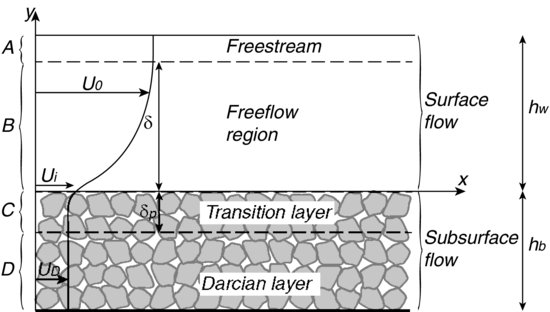
Figure 4.2 Instantaneous wall-normal velocity fluctuations v′ over and within a cubically packed bed of spheres (two layers) in a selected streamwise/wall-normal (x, y) plane obtained using LES. Adapted from Stoesser et al. 2006, with permission from the authors.
The critical experimental data required to confirm these assumptions, and thus validate these models, do not exist, as flow within the porous wall has remained largely inaccessible to standard measurement techniques owing to complexities of the porous bed (Blois et al., 2012a). Measurements of pressure fluctuations collected inside natural sediment beds suggest that these fluctuations decrease exponentially with depth. Vollmer et al. (2002) found that 90% of the high-frequency fluctuations were dampened at y/dp = –4.5 (where y is depth in the bed and dp is a measure of particle diameter), whilst at y/dp = –9 no pressure fluctuations were present. These observations suggest that the transition in flow regime occurs very rapidly and that the transition layer is rather thin, being a few grain diameters in natural sediment beds. Vollmer et al. (2002) also found that high-frequency pressure oscillations vanished more rapidly than low-frequency fluctuations, suggesting that permeable walls act as low-pass filters. Vollmer et al. (2002) argued that high-frequency oscillations originate from small-scale turbulence in the surface flow, and reported no clear linkage between large-scale structures and low-frequency oscillations. As for flow velocities within the porous wall, few and largely contradictory experimental results have been reported (Prokrajac et al., 2007; Detert et al., 2007). Prokrajac et al. (2007) used ultrasonic Doppler velocimetry within a cubically packed bed of uniform spheres to measure the velocity at different depths within the bed, and found that the mean streamwise velocity did not decrease monotonically with increasing depth in the bed, but rather presented a maximum underneath the interface. Detert et al. (2007) found no clear profile shape when using low-resolution endoscopic PIV but proposed a logarithmic fit to interpret the highly scattered data.
The conceptual importance of the transition layer has been largely overlooked and, due to a lack of understanding of this layer, the theoretical framework established for turbulent boundary layers developed over impermeable walls is systematically employed for permeable beds. Herein, we stress that despite the relatively small thickness of the transition layer, the physics of flow in this layer cannot be neglected, because flow interactions occurring in this region govern the structure of the near-wall flow and, in turn, determine the global effects of permeability, as discussed further below.
4.3 Boundary layer structure in the freeflow region over permeable beds
It is well recognized that interactions across the interface of a permeable wall significantly alter the structure and dynamics of near-wall turbulence, irrespective of whether the surface-subsurface interface is smooth or rough. Due to relaxation of wall blockage, mass exchange between the turbulent surface and subsurface flow (Manes et al., 2011a) results in significant ‘injection’ (flow from the pore space to the outer flow) and ‘suction’ (flow from the outer flow into the pore space) events across the interface (Stoesser and Rodi, 2007; Suga et al., 2011). These turbulent events drive near-wall momentum exchange processes that are entirely different from those induced near impermeable walls, resulting in a significant increase in surface drag (Manes et al., 2011b) and thus higher rates of energy loss (Suga et al., 2011).
4.3.1 Macroscopic effects
The most intuitive and expected effect of bed permeability is to modify the mean shear in the freeflow region, as compared to flow over an impermeable boundary. The resulting impact on the mean velocity profile and friction factor fc (fc ≡ 2 · τ/(ρ · v2)) is still under investigation. Several authors (Lovera and Kennedy, 1969; Ruff and Gelhar, 1972; Zagni and Smith, 1976) have reported that porous walls yield a higher fc than topographically-equivalent impermeable walls, and that permeability increases the skin friction by as much as 30–40% (Kong et al., 1982; Zippe and Graf, 1983). More recently, Breugem et al. (2006) showed that fc is permeability dependent and scales with the permeability Reynolds number, ReK, and pointed out that ReK must be directly correlated to the turbulence penetration depth δp. Manes et al. (2011b) attributed the rise in fc to a progressively deeper shear penetration into the wall with increasing ReK, and introduced the concept of an ‘effective roughness’ that scales with δp, and is limited by the wall thickness.
This dynamic influence is associated with a kinematic effect reflected in modifications of the wall-normal profile of streamwise velocity. Several studies report that the freeflow region outside the permeable bed is characterized by a logarithmic mean streamwise velocity profile (Manes et al., 2011a), analogous to that observed in flow over impermeable walls. However, the von Kármán coefficient κ of this logarithmic layer for a permeable wall, characterized by a permeability K, is significantly smaller (κ ≅ 0.24-0.39) than values reported for impermeable walls (κ ≅ 0.39-0.41) and decreases with increasing ReK. Manes et al. (2011a) reported that κ decreases with increasing d/δ (where d is the virtual wall-normal origin position) and that, as d is a length-scale characteristic of shear penetration, d/δ is effectively the ratio of the inner and outer scales. The relationship between shear, d, and turbulence penetration has not been clarified and the definition of the origin zero-plane raises additional questions that cannot be addressed herein. For the objectives of this chapter, it is important to emphasize that the global effects discussed above are associated with significant modifications in the organization of near-wall turbulence, and can be viewed as the most evident proof of the importance of permeability on controlling the structure of the turbulent boundary layer.
4.3.2 Turbulence structure in the freeflow
One of the distinctive features of flow over permeable walls, including laminar flows, is that an inflection point can occur in the mean streamwise velocity profile (∂2U/∂y2 = 0) just below the interface. Analysis by Drazin and Reid (1981) reveals an instability condition for which such an inflection point exists, which can give rise to Kelvin–Helmholtz (K–H) type instabilities and thus large-scale vortical structures that dominate the near-wall region. Numerical results from a direct numerical simulation (DNS) conducted by Breugem and Boersma (2005) using a permeable bed of cubes (Figure 4.3) appear to support such a hypothesis. Figure 4.3 shows the differences between flow near a smooth impermeable bed (top of Figure 4.3) and near a permeable bed (bottom of Figure 4.3). Flow at the impermeable bed suggests the occurrence of longitudinal flow structures, while that over the permeable surface shows the presence of large vortical structures characterized by spanwise vorticity. It is widely accepted that for canopy-type permeable walls, the structure of flow at the interface is dominated by K–H-type instabilities (White and Nepf 2007; Ghisalberti, 2009; Nepf, 2012). However, the application of such a hypothesis to more densely-packed porous matrices remains only partially accepted due to a lack of experimental observations.
Figure 4.3 Instantaneous velocity field (u′, v′) over and within a packed bed of cubes in a selected streamwise wall-normal (x, y) plane obtained from DNS, showing the difference between the flow near a permeable bed made of cubes, at the bottom, and near an impermeable smooth wall, at the top. Adapted with permission from Breugem and Boersma, 2005. Copyright 2005, American Institute of Physics.

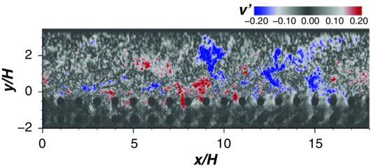
Figure 4.4 shows a typical instantaneous flow velocity field in the streamwise – wall-normal (x–y) plane over a porous bed of cubically packed spheres obtained herein using the surface flow PIV set-up illustrated in Figure 4.5. This data (see the animation video on the Wiley web site www.wiley.com/go/venditti/coherentflowstructures – data was collected at 20 Hz) illustrates the existence of spanwise vortices that persist over a long period of time while advecting downstream, similar to the coherent flow structures reported by Suga et al. (2011). The clockwise-rotating vortices are aligned along a diagonal line (Figure 4.4), and this organized configuration extends over a significant portion of the flow depth (i.e. freeflow region). In agreement with results of Stoesser et al. (2006), two main events are present near the bed: strong sweep (Q4) events, where higher momentum fluid is pushed towards the bed (u′ > 0, v′ < 0), together with ejection (Q2) events, where lower-momentum fluid is expelled away from the bed (u′ < 0, v′ > 0). These events govern the mechanisms of mass and momentum exchange that are responsible for energy loss across the bed. Despite the importance of these events in governing the mechanisms of surface-subsurface interaction and their implications in geophysical environments (e.g. incipient motion of grains at interface, biofilm growth, pollutant transport), experimental data capable of capturing the physics of these turbulent flows is lacking.
Figure 4.4 Instantaneous velocity field (u′,v′) over a cubically packed bed of spheres (six layers) in a selected streamwise/wall-normal (x, y) plane obtained using EPIV. The colour map refers to swirling strength (see Adrian et al., 2000b) expressed in s−1. Circles show clockwise-rotating vortices advecting downstream. The data were collected in the flume illustrated in Figure 4.5 using the surface flow PIV setup.
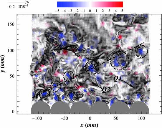
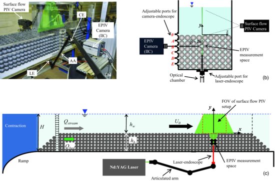
Figure 4.5 Experimental setup of the endoscopic PIV (EPIV): (a) Photograph showing the test-section that contains the packed bed and is instrumented with EPIV. In the top left of the picture, the camera used to measure the freeflow is also shown. (b) Endoscope configurations in the transverse section (width = 0.36 m) showing the setup of the endoscopes in the y-z plane. (c) Schematic diagram of the streamwise wall-normal (x, y) view of the flume test-section (length L = 2.80 m, height H = 0.60 m, slope θ = 0). Flow is from left to right; Qstream and Qbed refer to the mean flow discharge above and through the bed respectively (U0 is the mean depth-averaged velocity in the surface flow).
Additionally, recent investigations of flow over and through permeable walls (Packman et al., 2004; Blois et al., 2012a) have highlighted how the presence of small- and large-scale topography can dramatically enhance these interactions, thus modifying both the flow characteristics in the freeflow and in the transition layer. Since the beds commonly employed in past work were simultaneously rough and permeable (e.g. Manes et al., 2009; Blois et al., 2012a), the specific role of permeability in these processes often cannot be isolated. It is increasingly understood that the role of permeability can be quantified only using permeable walls that are perfectly smooth. This is challenging in experiments that use classical approaches to build the permeable bed (i.e. sediment, spheres). Recently, several new approaches have been proposed to overcome this limitation. Suga et al. (2010) and Manes et al. (2011a) attempted to minimize the effects of roughness, while enhancing permeability, by using smooth permeable walls. In particular, Suga et al. (2010) and Manes et al. (2011a) used foams (ceramic and polyurethane, respectively) that had a homogeneous and isotropic permeability structure with small filaments. Suga et al. (2010) reported that the onset of turbulence in the outer flow over a permeable bed occurred at a lower freeflow Reynolds number, Re (Re ≡ hw·Uo/ν), than over a smooth impermeable wall, and attributed this effect to permeability. However, despite the efforts of Suga et al. (2010) and Manes et al. (2011a) to eliminate the effects of roughness, the fine-scale texture of the foams still increased the flow resistance. Conversely, numerical approaches allow the imposition of perfectly smooth permeable walls, and thus permit the relative effects of roughness and permeability to be isolated. For instance, Breugem et al. (2006) modelled packed beds with relatively high porosity and small (nominally zero) particle diameters, and, by controlling these parameters, investigated the relative effect of each one on the flow structure.
Previous studies have highlighted several structural differences between flow over impermeable (ReK = 0) and highly permeable beds (high ReK), with one of the most striking being the disappearance of the near-wall, longitudinal, low- and high-speed streaks that occur in the buffer region of impermeable smooth-wall turbulence (Kline et al., 1967) and low permeability beds (Allen 1985). In addition, while wall-normal profiles of the Reynolds normal stresses (<u′2>, <v′2>, <w′2>) show clear peaks in the near-wall region, similar to smooth-wall flow, Breugem et al. (2006) found that permeability alters their magnitude. In particular, the peak value in the streamwise component of the Reynolds normal stresses (<u′2>/uτ2) decreased with increasing ReK, while that of the wall-normal (<v′2>/uτ2) and spanwise components (<w′2>/uτ2) increased. With increasing ReK, the peak value of the turbulent kinetic energy, TKE = 0.5 (<u′2> + <v′2> + <w′2>), decreased while the total shear stress increased, primarily due to enhanced Reynolds shear stress, <u′v′>. These results suggest that even at relatively-low Re (Re = 5.5 × 10³), the 3D nature of the flow plays a crucial role in energy transfer across a permeable wall. The higher-Re (Re = 3 – 9 × 10⁵) experiments of Suga et al. (2010) and Manes et al. (2011a) over quasi-smooth permeable walls revealed similar trends. Quadrant analysis by Manes et al. (2011a) over permeable walls revealed a near-wall region dominated by intense sweep events (Q4) and an outer region marked by weaker ejection events (Q2), in contrast to flow over impermeable walls that is typically marked by intense Q2 events (Wu and Christensen, 2006, 2007, 2010). Suga et al. (2011) also reported that permeability enhanced the intensity and duration of Q2 and Q4 events and found their observations to be ReK dependent, with an enhancement of Q4 events, especially near the wall, and a reduction in Q2 events as ReK increased.
It is well established that the transport of energy and momentum in smooth-wall turbulence is driven by the presence of large-scale coherent motions, termed hairpin vortex packets (Adrian et al., 2000a; Christensen and Adrian, 2001; Natrajan and Christensen, 2006; Ganapathisubramani et al., 2003; Adrian, 2007, Adrian, Chapter 2, this volume). These packets comprise a series of hairpin-like vortices that advect coherently, and their collective induction generates a region of relatively low streamwise momentum due to the ejection of low-speed fluid away from the wall. These large-scale vortex packets have also been observed in flows over rough, impermeable walls (Volino et al., 2007; Wu and Christensen, 2010), although their large-scale coherence appears mitigated slightly, particularly in the near-wall region. Using this overall structural taxonomy of turbulence over impermeable walls, Suga et al. (2011) proposed structural modifications that were caused by bed permeability, as revealed through a series of particle-image velocimetry (PIV) measurements of flow over ceramic foams with varying permeability. Using Galilean decomposition (Adrian et al., 2000b), Suga et al. (2011) detected the presence of coherent structures consistent with hairpin vortex packets. They also noted that, while the overall characteristics of these structures for low ReK were quite similar to those of flow over impermeable walls, their organization progressively decayed with increasing ReK. Suga et al. (2011) attributed this decay to the role of permeability in inhibiting the development of the hairpin legs due to enhanced vertical velocity fluctuations near the wall. For ReK >3, the energetic sweep events impinged on the hairpin heads toward the wall, while the weaker ejections could not sustain the organization of their legs. This decay in coherence provides an explanation for the absence of longitudinal low-speed streaks with increasing ReK. Suga et al. (2011) also argued that the existence of hairpin vortices does not contradict the occurrence of K-H structures, as the latter ‘could be superimposed onto the above events’ and may become dominant as ReK increases. Manes et al. (2011a) proposed a similar scenario, describing the phenomena as a ‘competing mechanism between shear instability eddies and attached eddies’, the latter of which are associated with hairpin packets whose size scales with the boundary-layer thickness, δ. Manes et al. (2011a) argued that permeability induces penetration of these eddies into the wall and triggers the production of shear instabilities that scale with the penetration depth δp. Thus, the dominance of one mechanism over the other is governed by the ratio δ/δp, whereby for high δ/δp attached eddies dominate whilst for low δ/δp K-H instabilities dominate.
4.4 Flow within the transition layer of permeable beds
4.4.1 Conceptual models
Classical models of flow over permeable walls can be divided into two groups: two- and one-domain approaches. In the former approach, independent sets of equations are used: the Navier–Stokes equations describe velocity in the outer-flow region while Darcy's equations are used for flow in the porous domain. This approach requires definition of both the location of the interface between the two domains and valid boundary conditions at this interface. While conservation of mass and pressure continuity are generally accepted boundary conditions, defining an appropriate interfacial velocity is problematic due to the differing order of the corresponding governing equations. A semi-empirical ‘slip’ boundary condition at the interface was proposed by Beavers and Joseph (1967) through the notion of a ‘slip coefficient’ α (i.e. an empirical dimensionless parameter) in conjunction with the mean streamwise velocity gradient just above the interface (y = 0+) as dU/dy ≡ α/K−0.5·(Ui - UD), where Ui is the velocity at the interface, known as the slip velocity. Independent measures of Ui, UD and K, yielded estimates of α. The analytical solutions of Beavers and Joseph (1967) were shown to be in good agreement with their experiments by adjusting α in the range 0.1-0.4, depending on the nature of the porous layer. Taylor (1971) performed experiments using a grooved plate and found α in the range 1.3 to 7. The primary issue with this approach is conceptual as, while the velocity is continuous at the interface, the tangential shear stress is not (from Ui to UD), meaning that the velocity within the transition layer cannot be determined. In addition, determination of Ui is very sensitive to the location of the interface which is unknown a priori. An alternative, multidomain, approach uses the Stokes' equation in the outer flow and the Brinkman equation in the porous domain (i.e. an extension of Darcy's equation in which a second order term, μeff ·D2·U, is incorporated; where μeff is the effective viscosity – see Brinkman, 1947). Both continuity of velocity and stresses can be satisfied with this approach because the governing equations are of the same order. Nevertheless, μeff depends on the structure of the porous domain rather than the properties of the fluid. Regardless of the approach, defining appropriate boundary conditions at the interface is extremely difficult. Furthermore, experimental validation of Brinkman's equation is quite limited.
In the single-domain approach, the composite domain is treated as a continuum in which the porous domain is considered a pseudo-fluid. The transition from fluid to porous medium is achieved through a gradual spatial variation of permeability. This formulation is optimal for numerical simulations as it removes the need to define the interfacial conditions, although its application requires adaptive discretization schemes. For example, Le Bars and Worster (2006) used a single-domain Darcy–Brinkman formulation. The Darcy–Brinkman equation assumes that above the wall the pressure gradient is balanced by fluid-fluid interaction (i.e. Stokes' equation), while deep in the wall it is balanced by viscous dissipation against the solid matrix (Darcy's equation). In the transition layer, both mechanisms play a role. The Darcy–Brinkman formulation predicts an exponential decay of velocity into the wall and, if the results are compared to Beavers and Joseph (1967), the velocity estimates converge in the pure fluid and deep into the wall, while the differences are obvious in the viscous transition zone where the latter involves a sharp transition.
4.4.2 Experimental observations of coherent flow structures in the transition layer and their evolution
The observations presented above clearly indicate that freeflow turbulence crosses the interface and penetrates to a significant depth in the porous domain, thus creating a more complex transition layer than has commonly been appreciated. The large, outer-layer eddies present in the turbulent boundary layer are typically blocked by the wall as long as their scale exceeds that of the characteristic pore space size. Within the porous wall, pressure (Vollmer et al., 2002) as well as velocity fluctuations (Manes et al., 2011a) vanish dramatically, undergoing a transition to a laminar state. In the transition layer, as suggested by the results of Stoesser and Rodi (2007), momentum is transferred from the freeflow to the pore flow through turbulence and from the pore flow to the solid matrix by viscous effects. Thus, the interaction between the freeflow and pore flows is mutual and complex and cannot be fully captured numerically with continuum approaches, nor with classical theoretical models that do not embody the dynamics of pore-scale eddies (Brinkman, 1947; Beavers and Joseph, 1967). Recent experiments in submerged, packed beds at high-Re (Pokrajac et al., 2007; Blois et al., 2012a) have highlighted that the transition layer of a permeable bed underlying a turbulent flow may be more complex than that postulated by the theoretical models outlined above. Momentum exchange at the interface may result in nonmonotonic vertical profiles (Pokrajac et al., 2007) and in a complex mean-flow structure.
Blois et al. (2012a) provided a number of quantitative visualizations using a novel endoscopic PIV (EPIV) experimental approach that allowed the complexity of the instantaneous flow fields within an individual pore space to be captured. The experimental set-up consisted of two borescopes, one to image the pore space and one to illuminate it (Figure 4.5). The camera-endoscope (CE) was 300 mm long with an 8 mm external diameter shaft borescope equipped with an imaging lens with variable focus adjustment. The laser endoscope (LE) consisted of a 270 mm long probe (12 mm external diameter) that terminated at an 8 mm diameter cylindrical lens. The LE produced a light sheet that was 0.2–0.5 mm thick with a lateral divergence angle β ∼ 26°. The CE was connected to a 4 Mpixel image-intensified camera (IIC) and the LE was connected to a Nd:YAG laser through an articulated arm (AA). The camera-endoscope was inserted horizontally from the sidewall while the laser-endoscope was inserted vertically through the floor (Figure 4.5b). The full description of the experimental setup and methodology of these experiments is not reported here, and the reader is referred to Blois et al. (2012a) for additional details. These EPIV data showed that the flow can be strongly nonuniform, with regions of faster and slower moving flow resulting in significant velocity gradients and rotational flow. Blois et al. (2012a) also highlighted that existing theory for symmetrically bounded porous domains cannot describe the flow in the transition layer of a turbulent freeflow bounded by a permeable wall. In such a layer, mean pore-flow patterns show clear asymmetries in the streamwise and vertical components of velocity, as well as in the turbulence statistics. Here, we present data from one specific flow boundary condition: dp/hw = 0.21; Re = 2.1·104; Fr = 0.1 (where Fr ≡ U0(g·hw)−1/2). The mean pore-space averaged streamwise velocity for this case was Up = 0.012 ms−1. This gives a characteristic pore time-scale tp = 3.3 (where tp = Up/dp), which represents the mean time of transit of a particle across the entire pore space. The spatial resolution of this EPIV velocity field allowed observation of coherent flow structures in the pore space with a minimum size of approximately 1 mm (≈ 1/40th of the pore diameter). The temporal resolution of the EPIV (acquisition frequency = 7 Hz) permitted, for the case presented here, the temporal evolution of these coherent flow structures to be observed and temporally traced in their motion across the pore space.
A number of examples of such pore-space flow evolution are reported below in order to outline the different mechanisms of flow structure, which all have the common feature of being triggered by pulsating multidirectional jet flows. Jet flows can be horizontal, vertical or a combination of the two, within the pore space, with the temporal evolution of the pore flow being a function of the intensity, direction and duration of these jets.
Here, a characterization of the flow is presented based upon the detection of topological patterns, such as stable and unstable vortices and saddles (see Perry and Chong, 1987), which can be considered large-scale coherent flow structures. The use of streamline patterns to identify the location of particular points within the flow (named ‘critical points’, see Chong et al., 1990) has been widely adopted in past work (e.g. Perry and Chong, 1987, Vollmers, 2001) to elucidate the topological structure of the flow. Here, a streamline representation is used to reveal the presence of coherent topological patterns within the flow. Three types of topological flow feature can be identified using this methodology: (i) large-scale vortical structures, (ii) spanwise jets and (iii) streamwise convergence and flow bifurcations.
4.4.2.1 Large-scale vortical structures
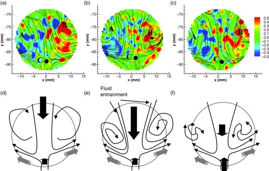
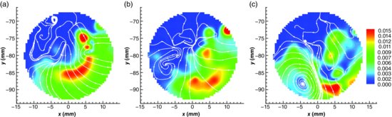
The first sequence (Figure 4.6) illustrates a quasi-vertical downward jet penetrating into a region of fluid that is initially moving slowly upwards. The downward jet flow results in rolling up of fluid and consequently generates vorticity within the pore space. Three steps can be recognized in the image sequence described topologically in Figure 4.6 (d, e and f): vortex formation, evolution and disorganization. The jet penetrating into the pore fluid produces vorticity on its sides (Figure 4.6d), with upward-moving fluid being deflected laterally and strengthening this further vortex evolution (Figure 4.6b). A saddle point (C) is observed at the junction of the jets that remains stable during the sequence reported here. The sequence in Figure 4.6 thus demonstrates the presence of stable, coherent, vortices, indicating considerable organization of flow in this pore-space. The mechanism of fluid entrainment that sustains this vortex development appears to be a shear instability, perhaps a Kelvin–Helmholtz instability, where the velocity gradient normal to the jet axis promotes fluid entrainment along its edges, thus bringing fluid from the top of the rotating regions into the swirling region, and thereby enhancing vortex development. The third phase in this development sequence (Figure 4.6c) shows the presence of unstable vortices that mark the end of the vortex growth mechanism and lead to the vortex disorganization phase and a reduction in spanwise vorticity. The observed lifetime, t, of vortical structures (in this case, t < 1 s) within the pore-space appears to be a function of the duration of the specific event that generates the vorticity. The dimensionless time of observation of the vortex, t* = t/tp, was t* ≈ 0.3. Termination of vortex development occurs when the downward jet flow ceases, possibly due to turbulent dissipation of the jet energy that is transferred to the fluid through the process of vortex formation.
Figure 4.6 Sequence of instantaneous flow fields within the pore space, showing three steps of vortex evolution driven by a downward-moving jet: (a) formation; (b) development; (c) disorganization. Panels (d), (e) and (f) show topological descriptions of the sequence: Black arrows represent fluid injected into the pore; grey arrows represent fluid ejection. In panels (a), (b) and (c) the colour map refers to vorticity and black lines represent streamlines. Freestream flow is from left to right.
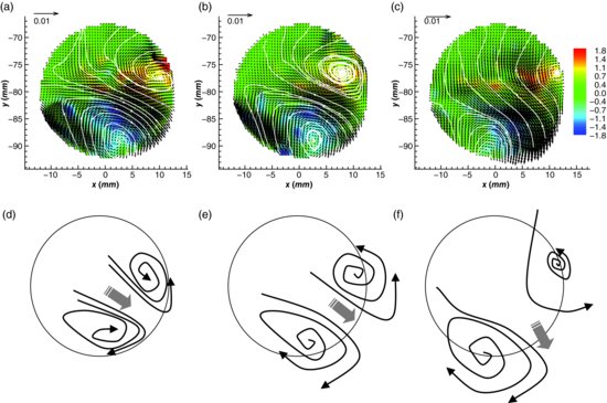
A similar, but slightly longer lived, phenomenon is illustrated in Figure 4.7, in which a diagonal jet within the pore space is observed flowing from top-left to bottom-right. For this event, the strength of the jet is high enough to produce much larger and persistent vortical structures. The vortex evolution described in Figure 4.7 is similar to that in Figure 4.6, with the formation of stable vortices (Figure 4.7a) being driven by shear instabilities that end when the velocity of the jet decreases (Figure 4.7b), and the vortices adopt an unstable configuration (Figure 4.7c).
Figure 4.7 Sequence of instantaneous flow fields within the pore space, showing three steps of the vortex formation process driven by a diagonal jet (from top left to bottom right). The colour map refers to the vorticity. White lines represent streamlines. Freestream flow is from left to right. Panels (d), (e) and (f) show topological representation of the vortex evolution.
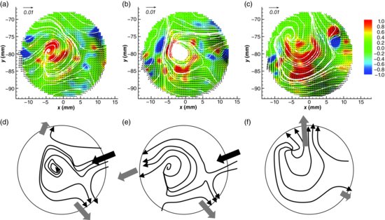
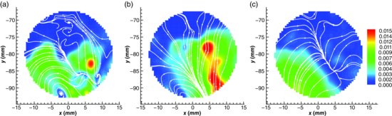
Additional examples of other longer events are reported in Figures 4.8 and 4.9, and show a quasi-horizontal jet first producing a counter-rotating vortex (Figure 4.8) and then sustaining its development (Figure 4.9). In this case, the jet is directed upstream and, in an earlier evolution stage is seen to produce a wavy path. This waviness indicates presence of a flow instability with smaller-scale vortices, with the jet introducing the energy required for production of larger-scale vorticity. The jet produces rotation and bending of the streamlines (Figure 4.8a and d), resulting in enhancement of vorticity within the sinuous streamlines and deviation of the point at which the flow exits the pore. Part of the flow exits at the bottom interconnecting pore throat (Figure 4.8b and e), which thus reduces ejection of fluid from the pore throat to the left of the image. This configuration subsequently promotes entrainment of fluid within the sinuous streamlines, resulting in formation of a stable vortex (Figure 4.8c and f). Further evolution of this vortex involves an increase in its strength (Figure 4.9a and d) and size before it begins to decay. The jet promotes production of positive vorticity and drives vortex evolution until it begins to become disorganized. Initially, the ejection of fluid occurs on the left and bottom sides of the pore space (Figure 4.9b and e). The stable initial vortex (Figure 4.8c) is sustained by fluid entrained within the circulation region from the bottom of the pore space, and this is visible until Figure 4.9a. From this point, the upper branch of the jet is deflected and fluid entrainment ceases (Figure 4.9c and f) and the vortex becomes unstable, wherein fluid, presumably from spanwise motion, is pushed away from the vortex along the streamlines and is finally ejected towards the top and bottom pores. In this example, vortex evolution can be tracked over 4 seconds, or t* ≈ 1.2. During this time, the vortex develops and moves slowly across the pore space before dissipating on the left side of the pore.
Figure 4.8 Sequence of instantaneous flow fields within the pore space, showing five steps of a counterclockwise vortex formation process driven by a downstream-moving jet. The colour map refers to the vorticity. White lines represent streamlines. Freestream flow is from left to right. Panels (d), (e) and (f) show topological representation of the vortex evolution.
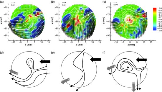
Figure 4.9 Sequence of instantaneous flow fields within the pore space, showing five steps of a counterclockwise vortex formation process driven by a downstream-moving jet. The colour map refers to the vorticity. White lines represent streamlines. Freestream flow is from left to right. Panels (d), (e) and (f) show topological representation of the vortex evolution.
4.4.2.2 Spanwise jets
Flow within the pore space is found to be highly 3D, with the pores exchanging mass and momentum in all directions, including the spanwise direction. Spanwise jets occur sporadically, as suggested by the recurrent presence of a 2D topological feature known as a ‘star’. These features are the degenerative form of a node and vortex (Perry and Chong, 1987) and indicate that the out-of-plane component of velocity may be sustaining the flow, thus suggesting the presence of spanwise jets. An example of a spanwise jet is given in Figure 4.10, which shows a region of low velocities surrounded by a region of radially-moving flow that possesses higher velocities (Figure 4.10a). This pattern of flow reflects the fact that the EPIV used herein can only quantify the components of velocity in the measurement plane, and a pure spanwise motion would thus produce zero particle displacements in the PIV measurements. For this reason, this low-momentum region at the top of Figure 4.10 is interpreted as the signature of a spanwise jet from a lateral pore throat that is directing fluid towards the pore, while the high-momentum region is interpreted as a roll-up of the jet that forms the spanwise vortex. This particular form of flow topology is known as a ‘repelling star’ (Perry and Chong, 1987) and is a degenerative form of an unstable spanwise vortex combined with an unstable node. The critical point (region) of this topological feature is its low momentum region, meaning that the jet is moving fluid from the centre of the pore toward the edges. When orthogonal jets interact with a rotating fluid mass, they may result in unstable vortices that are the degenerative form of a star. Moreover, if these jets interact with a quiescent or nonrotational flow, a typical degeneration of a star is shown by a streamline node. However, since spanwise jets are seldom perfectly orthogonal to the measurement plane, the degenerative topological features noted above are also observed.
Figure 4.10 Sequence of instantaneous flow fields within the pore space, showing four steps of activity of a spanwise jet forming a repelling star and, in consequence, large-scale vortical structures. The colour map refers to the velocity magnitude. White lines represent streamlines. Freestream flow is from left to right.
4.4.2.3 Streamline flow convergence and bifurcation
Another topological feature produced by the 3D nature of the pore flow, and observed in the present instantaneous streamline flow fields, is the bifurcation line. This topological feature is linked to unstable/stable nodes and is the line along which two flows of different direction meet. Figure 4.11 shows a stable bifurcation line along which the streamlines converge and the velocity magnitude is close to zero, suggesting that the flow is being deflected in an orthogonal direction. A conjunction line can also be identified (Figure 4.11) that separates two regions of different flow direction, which highlights the possible presence of counter-rotating vortices that have their axis parallel to the measurement plane (i.e. quasi-streamwise vorticity).
Figure 4.11 Sequence of instantaneous flow fields within the pore space showing four steps in the evolution of a bifurcation line. The colour map refers to the velocity magnitude. White lines represent streamlines. Freestream flow is from left to right.
4.4.3 Turbulence penetration into the bed: preliminary quantification using a novel refractive index matching (RIM) experimental approach
It is evident from the preceding discussion that the dynamic flow interactions across the transition layer at high-Re need to be better understood in order to determine how turbulence decays within the wall, which mechanisms transfer energy from large-scale structures in the surface flow to dissipative scales in the pore flow, and the nature of the linkage between turbulent events above and below the interface. Goharzadeh et al. (2005) used a refractive-index-matching (RIM) approach that allowed PIV measurements of flow to be collected within randomly-packed beds without the use of endoscopic probes. In their study, Goharzadeh et al. (2005) used borosilicate glass beads that were rendered optically transparent by this RIM approach but, due to the high kinematic viscosity of the working fluid (e.g. a special silicon oil mixture; νSilOil = 42.5 · 10−6 m2s−1), the investigation was limited to low-Re flows (Re ∼ 2 · 101) and thus no turbulence was generated.
A similar RIM approach has been used herein to conduct measurements at higher Re (Re ∼ 104–105) sufficient to generate turbulence in the freeflow, and preliminary results illustrating the great potential of this technique are shown below. The working fluid used was an aqueous solution of sodium iodide (NaI, 63% in weight) that has a high specific gravity (ρNaI/ρH2O ≈ 1.9) but its kinematic viscosity (νNaI = 1.1–1.5 10−6 m2s−1) is only 10–15% greater than that of water, thus allowing high-Re to be achieved. A specially designed flow facility was built to address the technical challenges of handling the NaI solution, which is highly corrosive and sensitive to oxygen and light exposure. The facility comprised a recirculating tunnel and a processor vessel to treat the NaI. The tunnel was fully pressurized with nitrogen (N2) and the temperature of the working fluid was controlled through an integrated system based upon a thermocouple, an in-line heat exchanger and an automatic modulating valve to control the flow rate of the cooling fluid. This allowed control of the temperature, and thus the index of refraction, of the NaI solution over long time periods and for the challenging conditions of high-Re flows. The acrylic test section (Figure 4.12) was 2.5 m long and had a square cross-section (0.1125 ·0.1125 m). Additional technical details of this new RIM facility developed for high-Re experiments are reported in Blois et al. (2012b).
Figure 4.12 Example of experimental setup to obtain accurate matching of the refractive index between the fluid and solid phases: (a) randomly packed bed of acrylic spheres, (b) partial immersion of spheres in NaI at ambient temperature; and (c) full immersion in temperature controlled flow at 18° C.
The experiments reported here were conducted using a flow rate Qtot = Qstream + Qbed = 3.3 L s−1, achieving ReH ≈ 3·104 (ReH ≡ ρ·U·H·μ−1, where H = 0.1125 m is the total depth of the tunnel and U is the mean velocity, U = Qtot/H2). The permeable bed used for the experiments reported herein was constructed of randomly packed acrylic (PMMA) spheres (Figure 4.12a), which in the present example were freely suspended in the NaI solution, with the pore-space flow being measured with PIV. To illustrate this, in Figure 4.12b the bed is partially immersed in the NaI solution at ambient temperature showing that the solid particles underneath the interface can hardly be seen. Difficulties arise at high Re. The index of refraction (RI) of the PMMA can be considered approximately constant (nPMMA = 1.4947) while the RI of the NaI solution was a function of temperature. At high Re flows, the temperature of the working fluids would increase quickly due to the high pump speed. However, by cooling the flow system, the temperature was maintained constant (18 °C). In such circumstances, the RI of the working fluid for a specific wavelength was kept very close (nNaI = 1.495 ± 0.003) to that of the solid phase, thus rendering the immersed solid phase nearly invisible, as illustrated in Figure 4.12c. Using coherent light (laser wavelength, λ = 532 nm), the RI matching was finely tuned to eliminate any effect of refraction (as shown in Figure 4.13a), which thus allowed unimpeded and unaberrated optical access to flow within the permeable bed. Silver-coated hollow glass spheres (mean diameter,  = 10 μm) with a density of 1.7 gcm−3 were used as PIV tracer particles, and particle images were collected along the spanwise centreline of the flow loop. A 12-bit, frame-straddle CCD camera (2048 × 2048 pixels) coupled with a 28 mm focal-length lens was used to image the flow, while a double-pulsed Nd:YAG laser (15 Hz and 120 mJ per pulse) provided coherent (λ = 532 nm) illumination. Optics were used to form a light sheet in the plane x, y (see Figures 4.12 and 4.13) that was wide enough to illuminate the entire flow around a group of spheres and to obtain a constant lightsheet thickness (∼1.5 mm).
Figure 4.13 (a) Photograph of light sheet traversing the flow through a randomly packed bed of PMMA spheres in the RIM facility. (b) A sample PIV image.
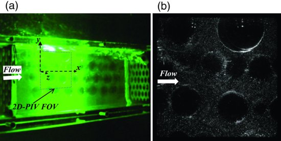
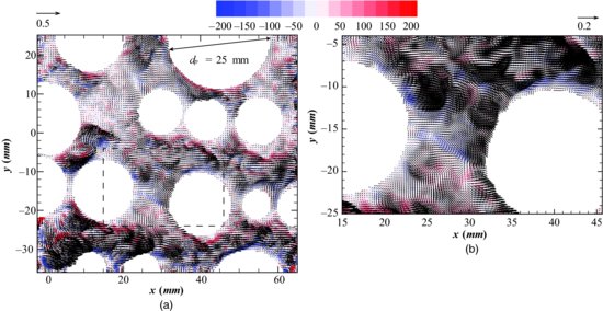
An example of the particle images obtained with this method is illustrated in Figure 4.13b, in which the circular dark regions correspond to the solid spheres. Interrogation of such images provides high-resolution instantaneous velocity fields, such as that shown in Figure 4.14, which illustrates the instantaneous velocity and vorticity distributions within a region of the packed bed. This velocity map shows that the high velocities in these pores produce flow separation at the surface of each sphere, thereby resulting in turbulent wakes that interact with the downstream spheres. These data highlight the ability of this RIM technique to quantify the turbulent flow generated by groups of spheres simultaneously, rather than limiting the visualization to an individual pore space. This technique will thus facilitate study of the complex mechanisms of flow interaction between adjacent pore spaces. Furthermore, the flow can be measured much closer to the fluid-particle interface that previous methods (including EPIV), thus allowing quantification of the interactions between pore flow and solid particles that is relevant for a number of geophysical flow applications (i.e. biofilm growth, fate of contaminant particles). Thus, this innovative experimental approach provides the ability to overcome the fundamental roadblock to proper interrogation of the flow dynamics across the flow-sediment interface and into the transition layer. In contrast to previous work, this optical access uniquely enables full quantification of the flow above and within porous beds with high spatio-temporal resolution via both planar stereo PIV and 3D volumetric PIV at high-Re. This will critically allow study of flow fields that are not yet computationally accessible, but are extremely relevant within many geophysical flows.
Figure 4.14 (a) Instantaneous PIV velocity field (u′,v′) within a randomly packed bed of spheres. The colour map denotes spanwise vorticity. (b) Zoomed-in view of dashed box region in (a), highlighting complex flow behaviour within the pore space and in the near-surface region around the spheres.
4.5 Discussion
Comparison of the coherent flow structures quantified in the present study to other experimental data is not possible since, to our knowledge, no equivalent experimental data exists. However, the LES results of Stoesser and Rodi (2007) provide an enlightening description of the interaction between the freeflow and pore-space flow. As suggested by Stoesser and Rodi (2007), the flow behaviour within the pore spaces is originally driven by the advection of large vortical structures in the freeflow that, as they form and translate downstream, generate alternate low- and high- pressure regions at the near-bed. We speculate that the resulting unsteady pressure distribution at the bed interface may then propagate through the bed, thus producing complex fluctuating local pressure gradients between the interconnected pores. Local pressure gradients are directly responsible for the unsteady interstitial flow observed herein and can be considered the main mechanism of energy transfer from the freeflow to the subsurface flow: energy is introduced into the pore by jet-like flows, and then dissipated by the turbulent processes observed in the present experiments. The strong inward and outward movements of fluid, numerically revealed by Stoesser and Rodi (2007), are observed in the present study in the form of local jets that are found to be the main driver of a number of complex flow patterns. The structure of flow within the pore space depends on several factors, and in particular on the characteristics of the pore space jets. Characterization of these jets in the present study has revealed several distinct forms of flow structure and turbulence dissipation, revealing new patterns of flow within porous media.
The observations summarized here (Figures 4.2 and 4.4) suggest that with increasing permeability (ReK), the momentum exchange processes of permeable-wall turbulence are governed by progressively more energetic sweeps that transport energy into the wall, and by a higher number of weaker ejections that transport back only a fraction of this energy. These processes therefore lead to a net loss of turbulent kinetic energy (TKE) from the outer flow to the pore flow, which is consistent with increased friction. Turbulent kinetic energy is dissipated inside the porous bed through mechanisms that remain largely unquantified due to a lack of experimental observations across the interface. This limitation has prevented the development of models that capture this crucial physics, and thus has stimulated the development of the new techniques detailed herein to overcome this fundamental hurdle to progress.
The essential ‘missing link’ to more fully understanding the physics of permeable-wall turbulence is the 3D unsteady interactions across the interface. Addressing this issue requires characterizing the flow not only above the wall, but also simultaneously deep within the wall to the turbulence penetration depth − the fundamental length scale of this problem. Indeed, Manes et al. (2011a) recently supported this notion from experimental evidence and stated that ‘the depth of shear penetration and the boundary-layer thickness should be taken as the characteristic inner and outer scales, respectively’. Likewise, recent numerical work concludes that turbulent interactions are sensitive to fluid velocity within the wall, meaning that progress in modelling requires quantification of these processes (Breugem et al., 2006). We contend that our poor understanding of permeable-wall turbulence is undoubtedly associated, at least in part, with a lack of experimental/optical access to the flow within a permeable wall due to its complex (typically opaque) nature. New developments using state-of-the-art optical diagnostics and experimental techniques clearly hold much promise for addressing these challenges.
4.6 Summary and challenges for future work
Flow in the presence of a permeable boundary is defined by: (i) a freeflow region, (ii) a transition layer and (iii) the Darcian layer. Flow within the Darcian layer is relatively simple and well described by Darcy's equation. Recent research has largely concentrated on quantifying the impact of a permeable boundary on the freeflow zone, which has revealed the following important differences to coherent flow structures commonly found over impermeable beds:
- The permeable boundary can act like an additional type of roughness, increasing skin friction by potentially as much as 30–40% as compared with an equivalent impermeable wall.
- There are significant interactions between the freeflow and transition layer driven by injection and suction events across the interface, which are absent in flow over an impermeable wall.
- While coherent near-wall flow structures are typically characterized by high- and low-speed streaks over an impermeable wall, these are largely absent in the presence of a permeable boundary.
- Permeable beds are characterized more by intense sweep (Q4) events, in contrast to impermeable beds that are more likely to be dominated by intense ejection events (Q2).
- Hairpin vortex structures seem to be present over both types of boundaries, although over permeable beds they become less distinct with increasing ReK.
The transition layer, between the freestream and Darcian layer, is the least well understood component of the permeable boundary environment and, largely due to logistical problems of experimental design, this layer has necessarily been treated quite simply, for example using the concept of a slip coefficient. However, recent technological advances using endoscopic particle image velocimetry and refractive index matching have revealed a much more complex hydrodynamic environment within the transition layer than has hitherto been realized. Coherent flow structures within pore spaces are primarily driven by pulsating multidirectional jet flows that generate the following typical features: (i) large-scale vortical structures, (ii) spanwise jets and (iii) streamwise convergence and flow bifurcations. Instantaneous flow data indicate that such features can be tracked within the pore spaces, here over periods of ∼1–5 s, or a dimensionless time t* of ∼0.3–1.5. These pore-scale structures are driven by exchange across the interface with the freeflow, and become more intense as the freeflow Re increases.
These recent results provide a tantalizing glimpse into the transition layer environment and indicate that current theories that are routinely employed in numerical treatments of this region are probably too simplistic. However, to capture fully the physics of this region requires more experimental data, most notably to answer the following questions: (i) How does turbulence decay within the transition layer, and how is this related to the bulk properties of the freeflow? (ii) What mechanisms transfer energy from large-scale coherent flow structures in the freeflow to dissipative scales in the pores of the transition layer? (iii) What is the nature of the linkage between turbulent events above and below the interface? The preliminary observations from several techniques reported here provide the basis for tackling these problems and generating comprehensive new experimental data. In order to properly answer these questions, simultaneous measurements of flow above and below the interface and in 3D are necessary: this is the challenge that must now be addressed.
4.7 Acknowledgements
We would like to thank the UK Natural Environmental Research Council for grant NE/E006884/1 that allowed development of the EPIV system, and the US National Science Foundation for award CBET-0923106 that has funded development of the RIM facility and award 1215879 concerning interfacial turbulence and hyporheic exchange. The authors also gratefully acknowledge the support of the International Institute for Carbon Neutral Energy Research (WPI-I2CNER), sponsored by the World Premier International Research Center Initiative (WPI), MEXT, Japan. We are also grateful to Ross Jackson for numerous discussions on coherent flow structures in many natural flows that have been inspirational for this chapter.
Notation
| AA | articulated arm to convey laser light |
| B | channel width [L] |
| CE | camera endoscope |
| fc | = τw/(ρU2), bed friction coefficient [-] |
| D | mean grain diameter [L] |
| dp | mean pore space diameter [L] |
| d | position of virtual wall-normal origin [L] |
| EPIV | endoscopic particle image velocimetry |
| Fr |  , Froude number [-] , Froude number [-] |
| g | acceleration due to gravity [L/T2] |
| H | cross-sectional averaged flow depth or flow thickness (including bed) [L] |
| hw | cross-sectional averaged flow depth or flow thickness |
| IIC | image-intensified camera |
| K | bed permeablity [L2] |
| ks | grain roughness height associated with skin friction [L] |
| L | length of test section [L] |
| LE | laser endoscope |
| nNaI | index of refraction of sodium iodide solution [-] |
| nSilOil | index of refraction of silicon oil [-] |
| p | pressure [M/L/T2] |
| PIV | particle image velocimetry |
| Q | flow discharge [L3/T] |
| Qbed | flow discharge through the bed [L3/T] |
| Qstream | flow discharge above the bed [L3/T] |
| Qt | = Qstream + Qbed, total flow discharge in the recirculating facility [L3/T] |
| Re | =  [-], flow Reynolds number [-], flow Reynolds number |
| Rep | =  [-], particle Reynolds number [-], particle Reynolds number |
| ReK | =  [-], permeability Reynolds number [-], permeability Reynolds number |
| RIM | refractive index matching |
| t | time [T] |
| tp | = Up/dp, pore-space time scale [T] |
| t* | = t/tp, dimensionless pore-space time [-] |
| Uo | depth- or cross-sectional-averaged flow velocity above the bed [L/T] |
| Ui | slip velocity (nonzero velocity at the interface) [L/T] |
| UD | = −K/μ ·(dp/dx), Darcy velocity [L/T] |
| u | streamwise component of flow velocity [L/T] |
| u′ | fluctuating component of streamwise flow velocity [L/T] |
| uτ |  , shear velocity [L/T] , shear velocity [L/T] |
| v | wall-normal component of flow velocity [L/T] |
| v′ | fluctuating component of wall-normal flow velocity [L/T] |
| w | spanwise component of flow velocity [L/T] |
 |
fluctuating component of spanwise flow velocity [L/T] |
| x | boundary-attached streamwise coordinate [L] |
| y | boundary-attached wall-normal coordinate [L] |
| z | boundary-attached upward spanwise coordinate [L] |
| α | slip coefficient, empirical coefficient parameter to estimate slip |
| β | optical divergence angle of laser endoscope |
| δ | thickness of turbulent boundary layer (freeflow) [L] |
| δp | depth of turbulence penetration into the bed [L] |
| κ | Kármán constant in logarithmic velocity profile [-] |
| λ | wavelength of PIV laser [L] |
| μ | dynamic viscosity of working fluid [M/L/T] |
| μeff | effective viscosity, empirical coefficient [M/L/T] |
| ν | kinematic viscosity of water [L2/T] |
| νNaI | kinematic viscosity of Sodium Iodide (NaI) solution [L2/T] |
| νSilOil | kinematic viscosity of Silicon Oil [L2/T] |
| ρ | water density [M/L3] |
| ρNaI | density of Sodium Iodide solution [M/L3] |
| θ | angle of inclination of bed [-] |
| τw | bed shear stress [M/L/T2] |
References
Adrian, R.J. (2007) Hairpin vortex organization in wall turbulence. Physics of Fluids 19, 041301, DOI: 10.1063/1.2717527.
Adrian, R.J., Meinhart, C.D. and Tomkins C.D. (2000a) Vortex organization in the outer region of the turbulent boundary layer. Journal of Fluid Mechanics 422, 1–54.
Adrian, R.J., Christensen, K.T. and Liu, Z.-C. (2000b) Analysis and interpretation of instantaneous turbulent velocity fields. Experiments in Fluids 29, 275–290.
Allen, J.R.L. (1985) Principles of Physical Sedimentology, George Allen & Unwin, London.
Beavers, G.S. and Joseph, D.D. (1967) Boundary conditions at a naturally permeable wall. Journal of Fluid Mechanics 30, 197–207.
Best, J. (2005) The fluid dynamics of river dunes: a review and some future research directions. Journal of Geophysical Research 110, F04S02. DOI: 10.1029/2004JF000218.
Blois, G., Sambrook Smith, G.H., Best, J.L., Hardy, R.J. and Lead J.R. (2012a) Quantifying the dynamics of flow within a permeable bed using time-resolved endoscopic particle imaging velocimetry (EPIV). Experiments in Fluids 53, DOI: 10.1007/s00348-011-1198–8.
Blois, G., Christensen, K.T., Best, J.L., Elliott, G., Austin, J., Garcia, M., Bragg, M., Dutton, C. and Fouke, B. (2012b) A versatile refractive-index-matched flow facility for studies of complex flow systems across scientific disciplines. 50th American Institute of Aeronautics and Astronautics (AIAA) Aerospace Sciences Meeting, Nashville, TN, AIAA Paper 2012-0736.
Boano, F., Revelli, R. and Ridolfi, L. (2007) Bedform-induced hyporheic exchange with unsteady flows. Advances in Water Resources 30, 148–156.
Breugem, W.P. and Boersma, B.J. (2005) Direct numerical simulations of turbulent flow over a permeable wall using a direct and a continuum approach. Physics of Fluids 17, 025103, DOI: 10.1063/1.1835771.
Breugem, W.P., Boersma, B.J. and Uittenbogaard, R.E. (2006) The influence of wall permeability on turbulent channel flow. Journal of Fluid Mechanics 562, 35–72.
Brinkman, H.C. (1947) On the permeability of media consisting of closely packed porous particles. Journal of Applied Sciences Research A1, 81–86.
Cardenas, M.B. and Wilson J.L. (2007) Dunes, turbulent eddies, and interfacial exchange with permeable sediments. Water Resources Research 43, W08412, DOI: 10.1029/2006WR005787.
Choi, H.G. and Joseph, D.D. (2001) Fluidization by lift of 300 circular particles in plane Poiseuille flow by direct numerical simulation. Journal of Fluid Mechanics 438, 101–128.
Chong, M.S., Perry A.E. and Cantwell B.J. (1990) A general classification of three-dimensional flow fields. Physics of Fluids A2, 765–777.
Christensen, K.T. and Adrian, R.J. (2001) Statistical evidence of hairpin vortex packets in wall turbulence. Journal of Fluid Mechanics 431, 433–443.
Darcy, H. (1856) Les Fontaines publiques de la ville de Dijon, Dalmont, Paris.
Detert, M., Klar, M., Wenka, T. and Jirka, G. (2007) Pressure- and velocity-measurements above and within a porous gravel bed at the threshold of stability. In Gravel-Bed Rivers VI: From Process Understanding to River Restoration (eds H. Habersack, H. Piégay and M. Rinaldi). Elsevier, Amsterdam, pp. 85–105.
Drazin, P.G. and Reid, W.H. (1981) Hydrodynamic stability, Cambridge University Press, Cambridge.
Finnigan, J. (2000) Turbulence in plant canopies. Annual Review of Fluid Mechanics 32, 519–571.
Ganapathisubramani, B., Longmire, E.K. and Marusic, I. (2003) Characteristics of vortex packets in turbulent boundary layers. Journal of Fluid Mechanics 478, 35–46.
Ghisalberti, M. (2009) Obstructed shear flows: Similarities across systems and scales. Journal of Fluid Mechanics 641, 51–61.
Ghisalberti, M. (2010) The three-dimensionality of obstructed shear flows. Environmental Fluid Mechanics 10, 329–343.
Goharzadeh, A., Khalili, A. and Jørgensen, B.B. (2005) Transition layer thickness at a fluid-porous interface. Physics of Fluids 17, 057102, DOI: 10.1063/1.1894796.
Kline, S.J., Reynolds, W.C., Schraub, F.A. and Runstadler, P.W. (1967) The structure of turbulent boundary layers. Journal of Fluid Mechanics 30, 741–773.
Kong, F.Y., Schetz, J.A. and Collier, F. (1982) Turbulent boundary layer over solid and porous surfaces with small roughness. NASA Contract Report NASA-CR-168990.
Le Bars, M. and Worster, M. G. (2006) Interfacial conditions between a pure fluid and a porous medium: implications for binary alloy solidification. Journal of Fluid Mechanics 550, 149–173.
Liu, Q. and Prosperetti, A. (2011) Pressure-driven flow in a channel with porous walls. Journal of Fluid Mechanics 679, 77–100.
Lovera, F. and Kennedy, J.F. (1969) Friction factors for flat bed flows in sand channels. ASCE Journal of the Hydraulics Division 95, 1227–1234.
Manes, C., Pokrajac, D., McEwan, I. and Nikora, V. (2009) Turbulence structure of open channel flows over permeable and impermeable beds: a comparative study. Physics of Fluids 21, 125109. DOI: 10.1063/1.3276292.
Manes, C., Poggi, D. and Ridolfi, L. (2011a) Turbulent boundary layers over permeable walls: scaling and near-wall structure. Journal of Fluid Mechanics 687, 141–170.
Manes, C., Pokrajac, D., Nikora, V.I., Ridolfi, L. and Poggi, D. (2011b) Turbulent friction in flows over permeable walls. Geophysical Research Letters 38, L03402. DOI: 10.1029/2010GL045695.
Natrajan, V.K. and Christensen, K.T. (2006) The role of coherent structures in subgrid-scale energy transfer within the log layer of wall turbulence. Physics of Fluids 18, 065104. DOI: 10.1063/1.2206811.
Nepf, H.M. (2012) Flow and transport in regions with aquatic vegetation. Annual Review of Fluid Mechanics, 44, 123–142.
Packman, A.I. Salehin, M. and Zaramella, M. (2004) Hyporheic exchange with gravel beds: basic hydrodynamic interactions and bedform-induced advective flows. Journal of Hydraulic Engineering 130, 647–656.
Perry, A. and Chong, M.S. (1987) A description of eddying motions and flow patterns using critical point concepts. Annual Review of Fluid Mechanics 9, 125–148.
Pokrajac, D., Manes, C. and McEwan, I. (2007) Peculiar mean velocity profiles within a porous bed of an open channel. Physics of Fluids 19, 098109. DOI: 19.1063/1.2780193.
Raupach, M.R., Finnigan, J.J. and Brunet, Y. (1996) Coherent eddies and turbulence in vegetation canopies: the mixing-layer analogy. Boundary Layer Meteorology 78, 351–382.
Ruff, J.F. and Gelhar, L.W. (1972) Turbulent shear flow in porous boundary. ASCE Journal of the Engineering Mechanics Division 98, 975–991.
Sahraoui, M. and Kaviany, M. (1992) Slip and no-slip velocity boundary conditions at interface of porous, plain media. International Journal of Heat and Mass Transfer 35, 927–943.
Stoesser, T, Fröhlich, J. and Rodi, W. (2006) Large eddy simulation of open-channel flow over and through two layers of spheres. Proceedings of the 7th International Conference on HydroScience and Engineering Philadelphia, USA, 10–13 September (ICHE 2006).
Stoesser, T. and Rodi, W. (2007) Large eddy simulation of open-channel flow over spheres. High Performance Computing in Science and Engineering 4, 321–330.
Suga, K., Matsumura, Y., Ashitaka, Y. et al. (2010) Effects of wall permeability on turbulence. International Journal of Heat and Mass Transfer 31, 974–984.
Suga, K., Mori, M. and Kaneda, M. (2011) Vortex structure of turbulence over permeable walls. International Journal of Heat and Mass Transfer 32, 586–595.
Taylor, G.I. (1971) A model for the boundary condition of a porous material. Part 1. Journal of Fluid Mechanics 49, 319–326.
Volino, R.A., Schultz, M.P., and Flack, K.A. (2007) Turbulence structure in rough- and smooth-wall boundary layers. Journal of Fluid Mechanics 592, 263–293.
Vollmers, H. (2001) Detection of vortices and quantitative evaluation of their main parameters from experimental velocity data. Measurement Science and Technology 12, 1199–1207.
Vollmer, S., Francisco, d.l.S.R., Daebel, H., and Kuhn, G. (2002) Micro scale exchange processes between surface and subsurface water. Journal of Hydrology 269, 3–10.
Whitaker, S. (1996) Advances in theory of fluid motion in porous media. Industrial and Engineering Chemistry 61, 14–28.
Whitaker, S. (1999) The Method of Volume Averaging, Kluwer, Dordrecht.
White, B.L. and Nepf, H.M. (2007) Shear instability and coherent structures in shallow flow adjacent to a porous layer. Journal of Fluid Mechanics 593, 1–32. DOI:10.1017/S00221120070084151
Wu, Y. and Christensen, K.T. (2006) Population trends of spanwise vortices in wall turbulence. Journal of Fluid Mechanics 568, 55–76.
Wu, Y. and Christensen, K.T. (2007) Outer-layer similarity in the presence of a practical rough-wall topography. Physics of Fluids 19, 085108. DOI: 10.1063/1.2741256.
Wu, Y. and Christensen, K.T. (2010) Spatial structure of a turbulent boundary layer with irregular surface roughness. Journal of Fluid Mechanics 655, 380–418.
Zagni, A.F.E. and Smith, K.V.H. (1976) Channel flow over permeable beds of graded spheres. ASCE Journal of the Hydraulics Division 102, 207–222.
Zhang, Q. and Prosperetti, A. (2009) Pressure-driven flow in a two-dimensional channel with porous walls. Journal of Fluid Mechanics 631, 1–21.
Zippe, H.J. and Graf, W.H. (1983) Turbulent boundary-layer flow over permeable and non-permeable rough surfaces. Journal of Hydraulic Research 21, 51–65.