10
Coherent Eddy Structures over Plant Canopies
ABSTRACT
For more than two decades, coherent flow patterns have been reported at the interface between vegetation canopies and the lowest levels of the atmospheric surface layer, a region called the roughness sublayer. Statistical analyses provided the first indications of such organization. Later, instrumented towers in forested lands revealed ramplike patterns in time traces of scalar quantities. When coupled with the velocity field measured by fast-response anemometry, a picture was formed of a repeated downstream ejection and upstream sweep combination creating streamwise convergence and the formation of scalar microfronts. Large-eddy simulation (LES) has been shown to reproduce both the statistics of canopy and roughness sublayer flow, and the turbulence structures detected in the field. Further, LES has allowed elucidation of the vortical nature of canopy flow structures and revealed a combination of head-up and head-down vortices, the former associated with the ejection and the latter with the sweep. Recent simulations that resolve flow within a forest canopy at the base of a full boundary layer under thermally unstable conditions illustrates the impact of surface heating on roughness sublayer structure and on mechanisms for heat, mass and momentum exchange at the surface. With increasing buoyant instability, momentum and scalar fluxes become increasingly disassociated in space. Convective cellular patterns produce regions of enhanced canopy-top shear and increased canopy drag beneath large-scale downdrafts. In updraft areas, canopy-top plumes coalesce to form the walls of the open-cell mesoscale structure, and diminished within-canopy drag.
10.1 Introduction
The exchanges of heat, water vapour, carbon dioxide and other gaseous and particulate matter between vegetation and the atmospheric surface layer have been the subject of intense interest for many decades. Studies of irrigation in agricultural lands and of carbon sequestration by the Earth's forests are among many that have demanded improvements in instrumentation and models of heat and mass transfer. In the belief that comprehension of the nature of turbulence at the interface is an essential step towards realistic modelling of surface/air exchange, great effort has been put into field, wind tunnel and numerical simulation of vegetation canopy and roughness layer flow. There is now the realization that coherent and repeated patterns of turbulent airflow make large contributions to the overall exchange of momentum and scalars between the atmosphere and managed and natural vegetated surfaces. Large-eddy simulation has proven to be a valuable tool in the study of canopy aerodynamics, and here we present results from simulations of both neutral and buoyantly unstable boundary layers.
10.2 Evidence for organized motion
Evidence for the existence and importance of coherent flow structures near rough surfaces and, in particular, plant canopies, has been provided by various statistical techniques. In quadrant analysis (Willmarth and Lu, 1974), the turbulent flux of momentum is partitioned into four quadrants based on the combination of signs of the perturbations of streamwise velocity u and vertical velocity w. Raupach (1981) showed a distinct difference in the characteristics of momentum transfer in flows over smooth and rough wind tunnel surfaces (as defined by the roughness Reynolds number) such that, over a smooth surface, momentum transfer is dominated by an outward ejection (Q2) of low momentum fluid away from the surface while, near a rough surface, Reynolds stress is dominated by a downward sweep (Q4) of high-momentum flow. Similar analyses using wind data from field studies in natural vegetation (Finnigan, 1979; Shaw et al., 1983) added confirmation of this distinction. The transfer of momentum into the canopy is dominated by sweeps of fast air from aloft but there is a transition to ejection dominance with increasing distance from the upper surface of the vegetation.
Further, streamwise and vertical velocity perturbations have been shown to be more strongly correlated near the canopy top, with correlation coefficients typically of the order of –0.5 compared to values of the order of –0.32 in the logarithmic layer sufficiently far from the plant surface (Finnigan, 2000). Such findings are strongly suggestive that fluid motions near the interface of a plant canopy are more organized than they are at greater heights. However, the statistics obtained by these analyses are global and do not offer direct information regarding the expected spatial and temporal coherence of flow structures, nor of their morphology.
10.2.1 Field observations
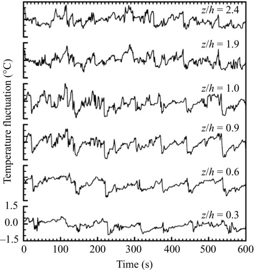
Demonstration of the existence of coherent structure in atmospheric turbulence at the interface with a canopy of vegetation appeared in the 1980s based on direct observations of airflow above and within tree canopies by fast-response anemometry (Denmead and Bradley, 1985; Gao et al., 1989; Bergstrom and Hogstrom, 1989). Using a vertical array of instruments deployed within and above a pine forest, Denmead and Bradley (1985) presented a sequence of temperature and humidity measurements to show the penetration of a vertically coherent gust of wind into the canopy. In a comprehensive study of canopy turbulence, Gao et al. (1989) showed a series of temperature fluctuations at six levels above and within a mixed deciduous forest. Sets of ramplike patterns (Figure 10.1), with gradually increasing temperature at each height terminated by a rapid fall, demonstrated that the thermal signal was vertically coherent but was witnessed first at the greatest height (2.4 times treetop height h in this case) and penetrated downwards towards the lowest reaches of the forest.
Figure 10.1 Ten-minute interval showing traces of temperature observed at six levels above and within a deciduous forest. Treetop height h = 18 m. Reproduced from Gao et al., 1989. With kind permission from Springer Science and Business Media.
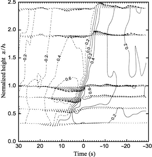
Combining both the scalar and vector fields, Gao et al., (1989) were able show the rapid transition from ejection of relatively warm and low momentum air from within the forest to a downward sweep of cooler, fast-moving air from aloft. They accomplished this by composite averaging sets of wind and temperature data centred on the rapid temperature drop at each height (Figure 10.2). The thermal pattern includes a sloping microfrontal boundary separating relatively warm and cool regions. Perturbation wind vectors relate closely to the scalar field with a strong sweep upwind of the microfront and a weaker ejection ahead of the microfront. Notice also the transition from sweep dominance near treetop height to ejection dominance at the level of the topmost instrument.
Figure 10.2 Composite average of ten ‘events’ detected by the rapid temperature drop of ramp patterns observed in a deciduous forest. Contour lines are of temperature departure (solid: positive; dash: negative) from the mean temperature at each level. Vectors are the u, w velocity perturbations. Time is reversed to give the impression of flow from left to right. Height is normalized by the treetop height h. Reproduced from Gao et al., 1989. With kind permission from Springer Science and Business Media.
The unusual character of turbulent flow in the roughness sublayer overlying vegetation canopies, as described above, led Raupach et al. (1996) to postulate that the plane mixing layer is a more appropriate model for roughness sublayer flow than boundary-layer flow. This was because the aerodynamic drag within the canopy maintains a vertical profile of streamwise velocity that includes an inflection point near the interface between the vegetation and the overlying free air, and hence an elevated shear zone. This proposal has gained much support since the 1990s.
10.2.2 Large-eddy simulation
The expense of erecting large arrays of fast-response anemometry and scalar sensors in a field environment initiated the application of large-eddy simulation (LES) to the problem of canopy flow (Shaw and Schumann, 1992). Nowadays, LES is used fairly commonly to simulate canopy flows. Generally, components of the vegetation are subgrid scale and their effects are parameterized in terms of element drag coefficients and scalar-source strengths, rather than being treated directly. Large-eddy simulation offers an additional significant advantage because the time-evolving three-dimensional flow field and pressure perturbations are computed directly. Static pressure measurements in the turbulent atmosphere are notoriously difficult because of the dynamic pressure perturbation, which appears around any instrument immersed in the flow. Observations of static pressure fluctuations at the ground surface are somewhat simpler, and Shaw et al. (1990) were able to demonstrate that a peak in static pressure accompanies and is coincident with the passage of scalar microfronts between ejections and sweeps. Thus, pressure pulses become useful and robust determinants of ramplike coherent structures.
The extraction of coherent flow patterns from LES of the canopy environment was first published by Fitzmaurice et al. (2004), with a 96 × 96 × 30 grid array representing a domain 192 m long, 192 m wide and 60 m high. The lowest ten grid intervals (20 m) or one-third of the vertical domain represented the vegetation with assigned element area densities and an appropriate drag coefficient at each grid point. Because of the extreme complexity of turbulent flows and the wide range of scales of motion contained therein, it proves useful to create composite averages of the events characterized by ejections, sweeps and scalar microfronts. Fitzmaurice and co-workers employed the positive pressure perturbations associated with such structures as the detection signal and aligned a large number of events with the centre of pressure perturbations detected at the canopy top (z = h). A similar analysis was performed by Watanabe (2004) but with a detection criterion based on the magnitude of the scalar microfront. The two studies yielded similar results in terms of the composite average vector and scalar fields.
Finnigan et al. (2009) published an equivalent but more extensive analysis, hereafter referred to as FSP. This study employed the National Center for Atmospheric Research LES, which uses pseudo-spectral methods in the horizontal, a second-order finite difference method in the vertical, and a third-order Runge–Kutta scheme for integration in time. The subfilter-scale stress tensor was estimated using the standard Deardorff (1980) formulation, as modified by Shaw and Schumann (1992) to account for enhanced dissipation due to canopy drag. Periodic boundary conditions were imposed in the horizontal directions. Analyses reported in this study relating to organized flow structures were based on runs with a domain of 1024 × 1024 × 128 uniformly spaced grid points, with the lowest ten grid intervals representing a 20 m tall vegetation canopy. The simulation was of a buoyantly neutral atmosphere. Sullivan and Patton (2011) and references therein provide further details regarding the inner workings of the LES code.
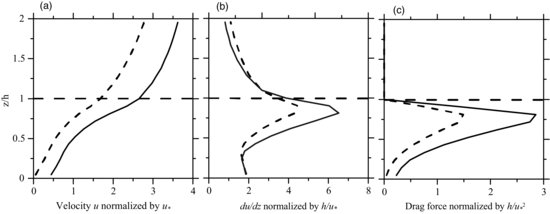
Figure 10.3 shows composite average perturbation fields of streamwise velocity u, vertical velocity w and of a passive scalar released by the canopy. The detection scheme was similar to that of Fitzmaurice et al. (2004) such that positive pressure perturbations at canopy top exceeding a suitably assigned threshold were used to identify and extract ejection/sweep structures. The figure shows contours of the three variables over an x,z slice through the centre of the composite average structure as defined by the peak positive pressure. Only the lowest portion of the domain is shown here, extending to three times the height of the canopy, while the streamwise dimension is truncated at a distance of plus and minus four times canopy height. The top section of the diagram showing the perturbation of the passive scalar illustrates a sloping microfront with a strong gradient separating high scalar concentration emitted from the canopy downwind of the centre, from low scalar concentration upwind. This portion of the figure should be compared with the temperature contours based on the field measurements presented in Figure 10.2. The close similarity between field observation and large-eddy simulation of the thermal pattern associated with coherent structures, together with the velocity pattern discussed below, provide justification for the use of numerical methods in this application.
Figure 10.3 Plots of passive scalar perturbation (top), vertical velocity perturbation (middle), and streamwise velocity perturbation (bottom) from a composite average of structures extracted from a buoyantly neutral LES, and detected using pressure peaks. Streamwise displacement rx/h is measured from the centre of the structure as determined by the centre of the positive pressure pulse at z = h and is normalized by the depth of the canopy. In each case, positive values are shown in red with solid contours. Negative values appear in blue with dash contours.
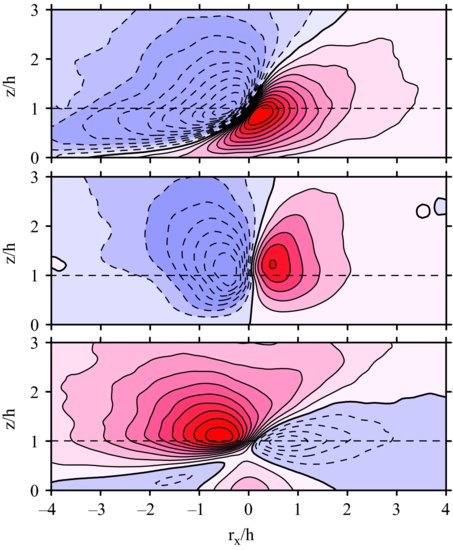
The central section of Figure 10.3 includes an updraft downwind of the pressure maximum and a downdraft upwind of peak pressure. The magnitude of vertical velocity in the downdraft exceeds that of the updraft. Unlike the scalar, which exhibits a tilt in the downwind direction, vertical velocity is reasonably vertically coherent. Vertical coherence in the vertical velocity had been demonstrated earlier by two-point correlation analyses in field studies (Shaw and Zhang, 1992), in a wind tunnel (Shaw et al., 1995) and in a large-eddy simulation (Su et al., 2000). Thus, vertical coherence of vertical velocity is revealed by both global statistics and by individual flow structures.
In the bottom section of the figure, streamwise velocity exhibits a somewhat more complex arrangement. In the upper portion of the canopy and in levels above canopy top, sweep and ejection regions are apparent with strong negative relationships between streamwise and vertical velocities. One major difference from the pattern of vertical velocity, though, is that the boundary between negative and positive streamwise velocity perturbation tilts in the downwind direction. Again, the positive streamwise velocity perturbation in the upstream sweep region is a stronger signal than that of the negative perturbation ahead of the pressure maximum within the ejection. In the lower half of the canopy, the pattern is quite different. In the centre of the structure, where we might have expected lower than average longitudinal velocity, we find a local maximum velocity. Since the streamwise location of this maximum coincides with that of the pressure perturbation, it is very likely that this is a consequence of pressure forcing in the bottom levels of the canopy, where the transfer of momentum from aloft is minimal.
Vector plots of lateral velocity v and vertical velocity w are shown in Figure 10.4, which has been reproduced from FSP at two streamwise displacements: one within the downdraft region and one within the updraft zone. In each case, we observe counter-rotating vortices displaced about plus-or-minus one canopy heights laterally from the centreline. Though not shown here, but illustrated by FSP, these vortex pairs increase in elevation as one progresses in the streamwise direction through both the sweep and the ejection portions of the structure. The authors attempted to illustrate the slopes of the vortices by plotting iso-surfaces of λ2, a quantity which was proposed by Jeong and Hussain (1995) as a definition of a vortex based on the eigenvalues of the symmetric tensor S2 + Ω2, where S and Ω are the symmetric and asymmetric parts of ∂ui/∂xj. Unfortunately, λ2 values are biased towards regions of high vorticity and are not coincident with the visual centres of rotating vortices shown in Figure 10.4.
Figure 10.4 Vectors of lateral and vertical velocity v, w across lateral traverses at approximately 0.8 canopy heights upstream (top, within the sweep), and downstream (bottom, within the ejection) of the centre of the composite average structure shown in Figure 10.3. Vectors are not to scale.
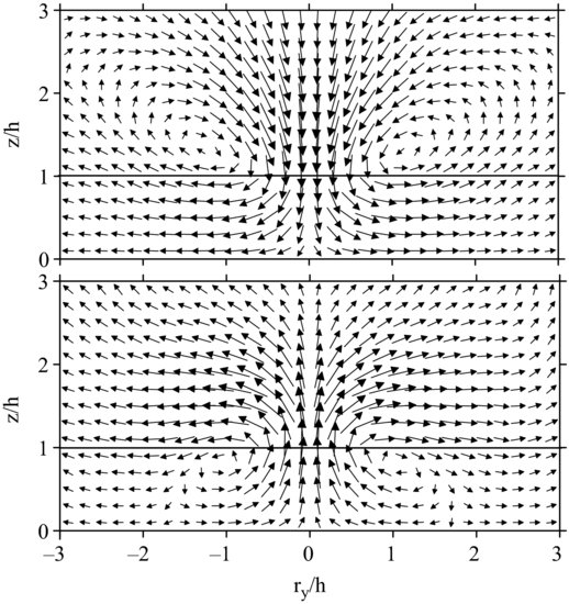
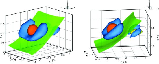
Figure 10.5 reproduces part of Figure 10.6 from FSP and shows the composite average structure from two different viewing angles. Vortices are represented in blue by iso-surfaces of λ2 appearing in two separate regions: one upwind and one downstream of the strong scalar gradient shown by the translucent sheet of green. Iso-surfaces shown in orange and yellow are of the magnitude of the composite average u′w′. The picture we get is of an upstream sweep (Q4) with strong downward motion between a head-down hairpin vortex (iso-surface of u′w′ appearing in orange), and a downstream ejection (Q2) with a weaker updraft between the legs of a head-up vortex (iso-surface of u′w′ appearing in yellow). In this example of the head-up vortex, the λ2 iso-surfaces do not appear to join at the head because the same λ2 value was used for both the sweep and for the weaker ejection. In any case, the λ2 plots are based on perturbation velocity. Had total vorticity been represented, we would expect the vortex cores to exhibit closed loops around each of the heads.
Figure 10.5 Three-dimensional representation of a coherent structure as a composite average of a large number of events identified according to a positive pressure pulse in the vicinity of the canopy top. The structure is shown from two directions in the right rear quadrant, as shown by the coordinate system at the upper right of each part. The isosurfaces shown in blue are of λ2 at a value of −0.77. The translucent sheet in green is an isosurface of zero scalar concentration perturbation from the horizontal average. The isosurface shown in orange is of u′w′ at a value of −0.6 m2s−2 in the region of the sweep, while that in yellow is the same quantity at a value of −0.15 m2s−2 associated with the ejection.
10.2.3 A model for vortex generation
Finnigan et al. (2009) compared the head-up and head-down vortex combination with hairpins found in the homogeneous shear flow simulations of Rogers and Moin (1987) and Gerz et al. (1994), which showed head-up and head-down hairpins occurring with equal frequency. In the latter case, head-up and head-down hairpins appeared in conjunction with one another, as in the FSP canopy simulation. In contrast, smooth-wall boundary layers generally only produce wall-attached head-up hairpin vortices (Tomkins and Adrian, 2003; Adrian, 2007). The distinction can be assigned to the fact that canopy flow induces a quasi-permanent elevated shear layer resembling that of a plane-mixing layer. FSP proceeded to develop a conceptual model for the creation of the paired head-up, head-down structures.
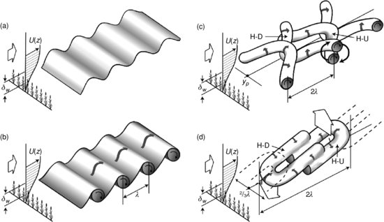
This model assumes that the coherent double-hairpin eddies are the end result of a cascade of linear and nonlinear instabilities, which is illustrated schematically in Figure 10.6. The first stage is the appearance of a train of transverse Kelvin–Helmholtz (K–H) waves, which are the linear eigenmodes associated with the inviscidly unstable inflected mean velocity profile at canopy top. They appear when the canopy top shear is enhanced by a downburst of higher momentum fluid of whole boundary layer scale. This increases the growth rate of the K–H waves, which is proportional to the mean shear, so they emerge from the background turbulence. These K–H waves evolve nonlinearly into transverse Stuart vortices spaced at the initial K–H wavelength,  . This train of Stuart vortices, in turn, is laterally unstable and random turbulent perturbations trigger the formation of trains of head-up and head-down hairpin vortices. Finally as the vortex pairs are deformed and stretched by the mean shear, the vorticity in their legs is amplified and self-induction causes the hairpins to remain closely superimposed. The upward motion through the legs of the downstream head-up hairpin forms a convergence zone with the downward flow through the legs of the upstream head-down hairpin. This convergence results in both the positive pressure pulse and the inclined microfrontal boundary of any scalar concentration exchanged with the canopy.
Figure 10.6 Schematic diagram of the formation of the dual-hairpin eddy: (a) The initial instability is a Kelvin–Helmholtz wave, which develops on the inflected mean velocity profile at canopy top. (b) The resulting velocity field is nonlinearly unstable and successive regions of alternating spanwise vorticity clump into coherent ‘Stuart’ vortices. (c) Two successive Stuart vortices are moved closer together at some spanwise location, by the ambient turbulence. The mutual induction of their vorticity fields causes them to approach more closely and rotate around each other. (d) As the initial hairpins are strained by the mean shear, most of the vorticity accumulates in the legs, and self-induction by the vortex legs dominates the motion of the hairpins.
10.3 Buoyancy forcing
Buoyancy forcing plays a vital role in geophysical turbulence, but was not included in the simulations of FSP. In an attempt to extend FSP's findings beyond neutral stability, a set of simulations varying the relative importance of buoyancy and shear has been completed (generated by varying the geostrophic wind). Levels of instability are specified according to the Obukhov length defined as:
(10.1) 
where  is the friction velocity, k is the von Kármán constant, g is gravity, and
  is the virtual potential temperature. Three simulations have been completed in which the Obukhov length ranged from L = −123 m (weakly unstable), through L = –32.5 m (moderately unstable) to L = –6.1 m (strongly unstable). A fourth run, without a mean wind, allowed for free convection.
The computational domain used 2048 × 2048 × 1024 nodes to resolve a physical volume 5120 × 5120 × 2028 m3 with grid spacing of 2.5 m in the horizontal directions and 2 m in the vertical. The forest resides in the lowest ten grid intervals, with a leaf area density that is horizontally uniform but vertically varying with a leaf area index of 2.0. The vertical profile of leaf area density was arbitrarily designed to create a relatively open understory and a relatively dense overstory. An element drag coefficient Cd = 0.15 was chosen on the basis of analysis of observations taken within a deciduous forest (Shaw et al., 1988). Sensible and latent heat transfers between the vegetation and within-canopy air were established at every time step using a model (unpublished) of a biologically and thermally active forest canopy subject to incoming solar and longwave radiation. The initial virtual potential temperature profile was constant (300 K) between 0 < z/h < 2, and then increased at a constant rate 3 K/km above z = 2h. The convective boundary layer developed up to heights between 670 and 800 m.
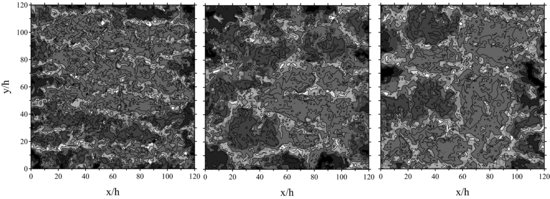
In the unstable boundary layer, an additional level of organization immediately becomes apparent. Large convective cells or eddies appear, spanning the full depth of the boundary layer and with horizontal extent of the order of 20 to 50 times the canopy height. Such scales are at least an order of magnitude greater than those of the turbulence created by canopy-top shear. These large-scale motions are evident even in the surface layer and close to the canopy top, as illustrated in Figure 10.7 showing contours of vertical velocity at z/h = 4 over one-quarter of the horizontal domain for the three levels of instability. In the weak instability case, there is evidence of streamwise elongation to the regions of upward motion, with longitudinal scales appearing to be greater than those in the lateral direction. This horizontal anisotropy is effectively eliminated with increasing levels of instability, and there is a tendency towards an open cellular pattern. The organization matches that found in LES simulations of the planetary boundary layer over a similar range of stability by Moeng and Sullivan (1994) and, in the free convection case, matches those presented by Schmidt and Schumann (1989).
Figure 10.7 Contours of vertical velocity at z = 4h for three levels of instability: left, weakly unstable (L = –123 m); centre, moderately unstable (L = –32.5 m); and right, strongly unstable (L = –6.1 m). In all cases, updrafts are shaded light, and downdrafts dark.
10.3.1 Similarity of momentum and scalar transport
Li and Bou-Zeid (2011) reported observations of fluxes of momentum, heat and humidity from tower measurements over a lake and over a vineyard, and found an increasing dissimilarity between momentum and scalar fluxes as the surface layer became more and more buoyantly unstable. Considering the quantities u′w′ and w′c′ as functions of time, where u and w are streamwise and vertical velocity and c is a scalar, they examined the correlation between the turbulent fluxes as defined by:
(10.2) 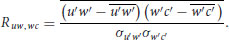
In their case, from tower observations of velocity, temperature and humidity, the overbar refers to a time average. They found a progressive decrease in the magnitude of the correlation coefficient for both heat flux and humidity flux with increasing instability, as defined by the negative of the ratio of the height above the surface to the Obukhov length, −z/L. There was considerable scatter in their data but, generally, the correlation coefficient fell from around –0.6 for the lake measurements and –0.5 for the vineyard study at –z/L = 10−2 to around –0.2 in both cases at –z/L = 1. The implication is that, at high levels of buoyant instability, momentum and scalars are transported by different eddies or at least by different parts of a flow structure, so that u′w′ and w′c′ are separated in time. There was little difference whether the scalar investigated was temperature or humidity.
We repeated Li and Bou-Zeid's (2011) analysis with the output from the large-eddy simulations. Using single realizations and performing correlations over the full horizontal domain, rather than over time, we found a similar loss of similarity between the flux of momentum and the fluxes of heat and humidity with increasing instability. Figure 10.8 shows profiles of the correlation coefficient between momentum flux and a scalar flux for the three unstable LES runs defined above, for the smaller domain neutral LES run used by FSP, and for the free convection LES run. For the neutral case, the scalar is passive while, for the other four cases, the scalar chosen is humidity, which participates in the buoyancy forcing. Under neutral and weak instability, the correlation coefficient is of the order –0.6 but, with increasing levels of instability, there is a clear degradation in the magnitude of the spatial correlation between momentum and scalar fluxes reducing to around -0.1 under strongly unstable conditions.
Figure 10.8 Vertical profiles of the horizontal spatial correlation of the fluxes of momentum u′w′ and humidity w′q′. Profile (a) is for the neutral case reported by FSP in which the scalar is passive. Profiles (b), (c) and (d) are, in order, the weakly unstable, moderately unstable, and strongly unstable runs. Profile (e) is for the free convection run with no mean horizontal wind.
Above the canopy, the correlation coefficients remain relatively constant. This lack of variation with height in the correlations, at least up to z = 4h, represents either a departure from the results of Li and Bou-Zeid (2011) or suggests that –z/L is not an appropriate nondimensional quantity in this situation. Alternatives to employing the height above the surface z as a scaling variable might be the boundary layer depth zi or a scale associated with the rough surface. This is yet to be determined. It remains clear that momentum and scalar fluxes become increasingly decorrelated with increased buoyant convection but it is not known whether this spatial decorrelation arises because momentum and scalar are transported by distinctly different fluid motions, or by separate parts of the same structures.
10.3.2 Influence of boundary-layer scale circulations
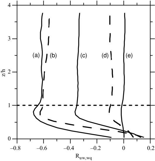
Planetary boundary layer structures partition the near-canopy flow into two distinct modes: (i) those below sinking regions where high momentum air is brought close to the surface and shear is high, and (ii) those below upwelling regions of the PBL-scale structures where near-surface wind is light and shear is small. Sinking and upwelling regions are defined according to the sign of the vertical velocity at z = 4h following application of a low-pass filter to the LES w-signal at that level, and are quite apparent in Figure 10.7. With this definition, for the moderately unstable run, rising motions occupy 48.5% of the horizontal domain, with the remaining 51.5% being occupied by sinking motions. Figure 10.9 shows vertical profiles of (a) the mean streamwise velocity in the roughness sublayer, (b) the corresponding streamwise velocity gradient, and (c) the drag force within the canopy corresponding to the two regions. In Figure 10.9, all variables are normalized using the domain-average friction velocity at the top of the canopy and the canopy-top height. The approximately 50% larger streamwise velocity beneath the regions of downwelling creates a similar increase in mean shear, and the increased momentum penetrating the canopy results in an approximate doubling of the drag.
Figure 10.9 (a) Mean streamwise velocity; (b) streamwise velocity gradient; and (c) drag force within the canopy, for the moderately unstable run (L = –32.5 m). In each case, the solid line represents calculations within downdraft regions and the dash line within updraft areas, as defined by the sign of the low-pass filtered vertical velocity at z = 4h. Canopy-top height h and the friction velocity u* calculated at z = h over the full horizontal domain are used for normalization.
Further information regarding the spatial disassociation of momentum and scalar fluxes can be educed by investigating the correlation coefficient separately in the updraft and downdraft regions. Above the canopy, in each of the three cases (weak, moderate and strong instability), momentum and scalar fluxes are more strongly correlated within the PBL-scale updrafts than downdrafts. For example, in the moderately unstable run, the spatial correlation coefficient between momentum and scalar fluxes in the updraft region is approximately –0.3 (just shy of the horizontal domain average value shown in Figure 10.8), but a value only around –0.1 in the downdraft region. Inside the canopy, this relationship reverses, with a stronger correlation in the downdraft but the correlations reduce to small negative or positive values near the ground surface in all cases. This sign reversal results from a reversal in the direction of the scalar flux since the upper canopy is the primary source of heat and vapour. The higher correlation in updrafts compared to downdrafts suggests that a different mechanism dominates turbulent transport in the two regions.
One might expect that, below regions of sinking motion where shear is large, the double-hairpin characteristic of the canopy shear instability would dominate vertical transport of momentum, with the sweep quadrant (Q4) being of greatest importance. In contrast, below the upward moving wall regions, where shear is weak, we should observe coherent convective canopy-scale plumes. These canopy-scale plumes would then coalesce to form the walls of the boundary-layer-scale convective cells. In these regions, the ejection quadrant (Q2) would dominate momentum transport near the canopy top and levels above the canopy.
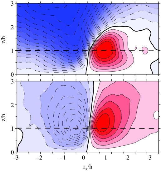
Without separating into PBL-scale updraft and downdraft regions, there is an apparent trend towards increased importance of sweeps relative to ejections as buoyant instability increases. For neutral and weakly unstable runs, triggering on positive pressure at the canopy top yields downdrafts with closed contours at canopy top or shortly above (Figure 10.3). However, with increasing instability, the downdraft strength continually increases with height up to at least z = 4h. On the other hand, the updraft downstream of the pressure pulse diminishes in importance but continues to be centred at or near canopy top. An illustration of this is presented in the top part of Figure 10.10 for the moderately unstable boundary layer. PBL-scale cellular patterns impose increased surface layer pressure below downdrafts because of (i) blocking by the underlying surface and (ii) a hydrostatic component due to the diminished temperature and humidity within the sinking motion. Applying a simple minimum pressure threshold as trigger for the detection procedure places additional emphasis on events within the downdraft region with the result that composites of canopy-top shear instabilities are overlaid with PBL-scale downdrafts.
To eliminate the influence of the PBL scales from the flow fields we high-pass (H-P) filtered all variables prior to compositing, with the intention of incorporating only canopy-scale motions in the resultant fields. The lower part of Figure 10.10 shows the result. Only minor differences appear between structures composited in this manner in buoyantly unstable conditions from those in Figure 10.3 for neutrally buoyant conditions. Further, though not shown here, little difference exists between structures extracted from H-P filtered fields beneath PBL-scale updrafts versus downdrafts.
Figure 10.10 Composite average vertical velocity from structures extracted using positive pressure perturbations as trigger. The top graph is without filtering while the bottom graph is with a high-pass filter applied to all variables, including the pressure at canopy top used for detection. Contour interval is 0.1 m/s in both cases. Solid lines are positive and dash lines negative vertical velocity.
Quadrant analyses (not shown) performed on the output from the unstable boundary-layer simulations support this interpretation because they do not show any significant change in the relative importance of sweeps and ejections. In all cases, sweeps (Q4) are most important within the canopy but ejections (Q2) become dominant shortly above the top of the canopy. It is clear that PBL-scale structures impose vertical motions that significantly impact transport processes throughout the roughness sublayer but details of how this is accomplished have yet to be revealed.
10.4 Summary and conclusions
Repeated organized flow structures are a significant aspect of turbulence within and immediately above a vegetation canopy, and contribute significantly to momentum and scalar exchange at such surfaces. Field, wind tunnel and numerical simulations basically agree in terms of both global and conditional statistics, and also in terms of the organized flow patterns of structures identified and extracted from real and simulated flows. An extensive examination of a large-eddy simulation under neutral conditions (Finnigan et al., 2009) showed the characteristic eddy to be comprised of a downwind head-up vortex and an upwind head-down vortex. Between the legs of the downwind vortex is an ejection of low momentum, scalar rich air, while a sweep of fast moving air from aloft lies between those of the head-down vortex. The resulting convergence occurring between the two vortices creates a sloping microfrontal boundary between air with high scalar concentration from canopy sources and fresh air from aloft. A proposal is presented in schematic form for the evolution of the head-up, head-down vortical structure.
Significant changes occur in boundary layer structure and in the horizontal distribution and nature of momentum and scalar fluxes at the canopy interface when convective instability brought about by solar heating of the vegetation and resulting positive sensible and latent heat fluxes are introduced. The first thing we notice is that fluxes of momentum and scalars become spatially decorrelated. While the quantities u′w′ and w′q′ are quite strongly correlated in a spatial sense under neutral and weak instability, this correlation is greatly diminished under conditions of strong instability.
To extract head-up/head-down structures under strongly convective conditions, it is first necessary to high-pass filter the flow variables to eliminate the increasing influence of PBL-scale circulations. Regions of downdraft enhance the streamwise velocity and shear near the canopy top and generate more active turbulence structures within and immediately above the vegetation.
10.5 Acknowledgements
Roger Shaw greatly appreciates travel support from both NCAR and CSIRO. Edward Patton acknowledges salary support from the National Center for Atmospheric Research's Bio-hydro-atmosphere interactions of Energy, Aerosols, Carbon, H2O, Organics & Nitrogen (BEACHON) project and from the Army Research Office (Grant No.: W911NF-09-1-0572) under subcontract from the University of Colorado, Boulder, and travel support from CSIRO Marine and Atmospheric Research. NCAR is sponsored in part by the National Science Foundation. This research used resources of the National Energy Research Scientific Computing Center, which is supported by the Office of Science of the U.S. Department of Energy under Contract No. DE-AC02-05CH11231.
References
Adrian, R.J. (2007) Hairpin vortex organization in wall turbulence. Physics of Fluids 19, 041301, 1–16.
Bergstrom, H. and Hogstrom, U. (1989) Turbulent exchange above a pine forest. II. Organized structures. Boundary-Layer Meteorology 49, 231–263.
Deardorff, J.W. (1980) Stratocumulus-capped mixed layers derived from three-dimensional model. Boundary-Layer Meteorology 18, 495–527.
Denmead, O.T. and Bradley, E.F. (1985) Flux-gradient relationships in a forest canopy. In The Forest-Atmosphere Interaction (eds B.A. Hutchison and B.B. Hicks). Reidel, Dordrecht, pp. 421–442.
Finnigan, J.J. (1979) Turbulence in waving wheat II. Structure of momentum transfer. Boundary-Layer Meteorology 16, 213–236.
Finnigan, J.J. (2000) Turbulence in plant canopies. Annual Review of Fluid Mechanics 32, 519–573.
Finnigan, J.J., Shaw, R.H. and Patton E.G. (2009) Turbulence structure above a vegetation canopy. Journal of Fluid Mechanics 637, 387–424.
Fitzmaurice, L., Shaw, R.H., Paw U, K.T. and Patton, E.G. (2004) Three-dimensional scalar microfront systems in a large-eddy simulation of vegetation canopy flow. Boundary-Layer Meteorology 112, 107–127.
Gao, W., Shaw, R.H. and Paw U, K.T. (1989) Observation of organized structure in turbulent flow within and above a forest canopy. Boundary-Layer Meteorology 47, 349–377.
Gerz, T., Howell, J. and Mahrt, L. (1994) Vortex structures and microfronts. Physics of Fluids 6, 1242–1251.
Jeong, J. and Hussain, F. (1995) On the identification of a vortex. Journal of Fluid Mechanics 285, 69–94.
Li, D. and Bou-Zeid, E. (2011) Coherent structures and the dissimilarity of turbulent atmospheric surface layer, Boundary-Layer Meteorology 140, 243–262.
Moeng, C.-H., and Sullivan, P.P. (1994) A comparison of shear- and buoyancy-driven planetary boundary layer flows. Journal of Atmospheric Science 51, 999–1022.
Raupach, M.R. (1981) Conditional statistics of Reynolds stress in rough-wall and smooth-wall turbulent boundary layers. Journal of Fluid Mechanics 108, 363–382.
Raupach, M.R., Finnigan, J.J. and Brunet, Y. (1996) Coherent eddies and turbulence in vegetation canopies: the mixing-layer analogy. Boundary-Layer Meteorology 78, 351–382.
Rogers, M.M. and Moin, P. (1987) The structure of the vorticity field in homogeneous turbulent flows, Journal of Fluid Mechanics 176, 33–66.
Schmidt, H. and Schumann, U. (1989) Coherent structure of the convective boundary layer derived from large-eddy simulation. Journal of Fluid Mechanics 200, 511–562.
Shaw, R.H., Brunet, Y., Finnigan, J.J. and Raupach, M.R. (1995) A wind tunnel study of air flow in waving wheat: two-point velocity statistics. Boundary-Layer Meteorology 76, 349–376.
Shaw, R.H., den Hartog, G. and Neumann, H.H. (1988) Influence of foliar density and thermal stability on profiles of Reynolds stress and turbulence intensity in a deciduous forest, Boundary-Layer Meteorology 45, 391–409.
Shaw, R.H, Paw U, K.T., Zhang, X.J., Gao, W., Den Hartog, G. and Neumann, H.H. (1990) Retrieval of turbulent pressure fluctuations at the ground surface beneath a forest. Boundary-Layer Meteorology 50, 319–338.
Shaw, R.H. and Schumann, U. (1992) Large-eddy simulation of turbulent flow above and within a forest. Boundary-Layer Meteorology 61, 47–64.
Shaw, R.H., Tavanger, J. and Ward, D.P. (1983) Structure of the Reynolds stress in a canopy layer, Journal of Climate and Applied Meteorology 22, 1922–1931.
Shaw, R.H. and Zhang, X.J. (1992) Evidence of pressure-forced turbulent flow in a forest. Boundary-Layer Meteorology 58, 273–288.
Su, H.-B., Shaw, R.H. and Paw U, K.T. (2000) Two-point correlation analysis of neutrally stratified flow within and above a forest from large-eddy simulation. Boundary-Layer Meteorology 94, 423–460.
Sullivan, P.P. and Patton, E.G. (2011) The effect of mesh resolution on convective boundary layer statistics and structures generated by large-eddy simulation, Journal of the Atmospheric Sciences 68, 2395–2415.
Tomkins, C.D. and Adrian, R.J. (2003) Spanwise structure and scale growth in turbulent boundary layers. Journal of Fluid Mechanics 490, 37–74.
Watanabe, W. (2004) Large-eddy simulation of coherent turbulence structures associated with scalar ramps over plant canopies. Boundary-Layer Meteorology 112, 307–341.
Willmarth, W.W. and Lu, S.S. (1974) Structure of the Reynolds stress and the occurrence of bursts in the turbulent boundary layer. Advances in Geophysics 18A, 287–314.