11

SPIV Analysis of Coherent Structures in a Vegetation Canopy Model Flow

Laurent Perret & Tony Ruiz

LUNAM Université, Ecole Centrale de Nantes, LHEEA, France

ABSTRACT

Coherent structures in the turbulent boundary-layer developing over a vegetation canopy are investigated. Attention is concentrated on the spanwise component and its role in the dynamics of the well-recognized sweep and ejection events associated to hairpin-like coherent eddies. A wind-tunnel experiment is performed and stereoscopic particle image velocimetry is used to measure the three components of the velocity in two different planes. One- and two-point statistics of the velocity show the high level of fluctuation of the spanwise component and that ejections and sweeps are linked by a spanwise motion that occurs below. Conditional average velocity fields based on the occurrence of ejections and sweeps combined with a nonzero spanwise velocity show that this spanwise coherent motion goes preferentially from the high-speed to the low-speed region. Spanwise fluctuations are also found to be involved in very large-scale structures consisting of low- or high-momentum regions, elongated in the streamwise direction and which meander in the horizontal plane. The present findings suggest a spatio-temporal organization of the coherent structures based on the hairpin vortex packets model, in which the spanwise component constitutes a dynamical link between sweeps and ejections but also affects the turbulence structure at a larger scale.

11.1 Introduction

The importance of coherent eddies in the turbulence structure of flows over and in vegetation canopies has been demonstrated by several past studies (see for instance Raupach et al., 1996; Finnigan, 2000; Dupont and Brunet, 2009; Finnigan et al., 2009). These coherent structures have been shown to play an important role in momentum transfer and in turbulence production, being major contributors to time-averaged turbulence statistics. When compared to boundary-layer over smooth walls, the presence of the canopy leads to a strong modification of the flow near the wall. An analogy with plane mixing-layer flows has been proposed to describe the structure of the flow, the dynamics of which has also been found to be dominated by large coherent structures (Raupach et al., 1996; Finnigan, 2000). In the roughness sublayer, sweeps rather than ejections dominate eddy-fluxes whereas it is the opposite above, where the flow recovers a structure similar to the one of canonical boundary layers populated by hairpins-like vortices arranged along low and high-momentum regions that form, in turn, larger scale structures (Adrian, 2007). Finnigan et al. (2009) proposed a new organization by showing that, at the top of the canopy, the characteristic eddy consists of an upstream head-down sweep-generating hairpin vortex superimposed on a downstream head-up ejection-generating hairpin. In their numerical study, Dupont and Brunet (2009) investigated the development of coherent structures from the canopy edge in the roughness sublayer and showed statistical similarities but also differences from an instantaneous point of view with the development of a mixing layer. Moreover, they deduced from the analysis of the two-point correlation tensor of the three velocity components, well downwind from the edge, the presence of two counter-rotating streamwise vortices around the sweep motion at the canopy top, interpreted as representing an ensemble average of the counter-rotating longitudinal vortices constituting the pair of hairpin vortices described by Finnigan et al. (2009).

Recent work from Hutchins and Marusic (2007) and Hutchins et al. (2011) has demonstrated the existence of a regime of very long meandering positive and negative streamwise velocity fluctuations in the log and the lower wake regions of a turbulent boundary-layer over a flat plate. These structures, termed ‘superstructures’, because of their streamwise length that can exceed 20 times the height of the boundary-layer δ, were evidenced by the large-scale stripiness in the longitudinal velocity fluctuations that they measured with a spanwise rake of ten hot-wires, and were found to scale with outer length variables δ. These spanwise meandering structures were also found in their experiments performed in a neutrally stable atmospheric surface layer. Hutchins and Marusic (2007) showed that the near-wall small-scale turbulence was influenced by the meandering superstructures. This was confirmed by Hutchins et al. (2011) in their study of the relationships between the large-scale superstructures and the skin friction events at the wall.

The existence of very large-scale structures in turbulent flows over canopies has also been the subject of recent studies. Using a spanwise array of sonic anemometers, Inagaki and Kanda (2010) studied the structure of turbulence over an array of cubes within the logarithmic layer of the atmospheric boundary layer and observed very large streaks of low momentum fluid elongated in the streamwise direction. They also identified two-modes in the spectrum of the longitudinal velocity which they were are able to separate using a filter in the spanwise direction: a high frequency mode that follows the inner scaling similarity, and a low frequency mode, expected to have an outer layer length scale and to be nearly inactive to the local Reynolds stress. They also reported that this low-frequency mode, which seems to share common features with the superstructures identified by Hutchins and Marusic (2007), also affects the spanwise component, in agreement with the meandering motion. The interaction between inner and outer layer structures in a convective boundary layer over an urban-like surface have been studied via large eddy simulation (LES) by Castillo et al. (2011). They found that structures corresponding to outer layer scales consist of low and high momentum streaky structures which influence the location of ejections and sweeps. In their experimental study of turbulent boundary layers over permeable walls, Manes et al. (2011) identified different types of coherent structure depending on the permeability of the wall. The higher the permeability, the more the near-wall flow resembles a perturbed mixing layer whereas very low permeability and smooth wall flows were characterized by a well defined logarithmic layer dominated by attached eddies. By means of spectral analysis, they also identified very large-scale motions in configuration of smooth and low permeability wall. Increasing the permeability led to a poor separation between inner and outer scales, making impossible of the detection of very large-scale motions via spectral analysis.

In the present study, coherent structures consisting of ejection and sweep motions, but also the presence of large-scale coherent structures meandering in the horizontal plane of a turbulent boundary layer over a vegetation canopy, are investigated by focusing on the fluctuations of the spanwise velocity component. This analysis is based on stereoscopic particle image velocimetry (SPIV) measurements performed in a wind tunnel over a canopy model made of rigid elements. Classical one-point statistics are first used to study the basic characteristics of the flow. Two-point correlations and conditional averages are then employed to investigate the imprint of the ejection and sweep motions on the spanwise component and their dynamics. The presence of very large motions is evidenced as well as their meandering feature in the horizontal plane. The outline of the chapter is as follows: Section 11.2 is devoted to the presentation of the experimental setup and procedure. Section 11.3 focuses on the results and the identification of the different coherent structures. In the last part, the structure of the flow and its spatio-temporal organization are summarized and discussed in details.

11.2 Experimental setup

11.2.1 Wind tunnel

Experiments were conducted in the atmospheric boundary layer wind tunnel of the LHEEA (Nantes, France), which has working section dimensions of 24 × 2 × 2 m. A suburban-type atmospheric boundary layer was generated upstream of the vegetation canopy model using a 13 m fetch of staggered cube roughness elements with a plan area density of 25%. The cubes height was h = 50 mm. The characteristics of the simulated urban boundary layer (friction velocity, height of displacement and roughness height) were found to be in good agreement with the literature (Cheng et al., 2007). The vegetation canopy model, described below, was located downstream this fetch of cubes. All the measurements presented here were obtained for a free stream velocity of 8.8 m/s.

11.2.2 Canopy model

In this study, an idealized vegetation canopy model was employed. It consisted of an array of staggered rigid cylinders, vertically standing, arranged in a regular pattern (Figure 11.1), located downstream of the initial 13 m fetch of staggered cubes. The height of the cylinders was h = 50 mm, and their diameter was dr = 4 mm, giving an aspect ratio of 12.5. The spacing between two cylinders in the same row was 32 mm and the distance between two rows was 16 mm. These dimensions led to a canopy density of n = 980 cylinders/m2 and a frontal area per unit volume a = n.dr = 3.92 m−1. The frontal area index of this staggered arrangement is . These geometrical parameters correspond to a dense canopy, deep enough to allow the existence of three distinct regions where, with increasing height from the ground, (i) the flow is dominated by the vortex shedding from the cylinders close to the ground, (ii) the mixing layer analogy holds near the canopy top and (iii) the flow resembles a displaced rough-wall boundary-layer above the canopy (Poggi et al., 2004).

Figure 11.1 Sketch of the vegetation canopy model installed downstream an initial 13 m fetch of staggered cubes. The canopy model was made of rigid cylinders (height: 50 mm, diameter: 4 mm) arranged in a staggered array. SPIV measurements were performed in two vertical planes located 120h downstream the start of the vegetation canopy model.

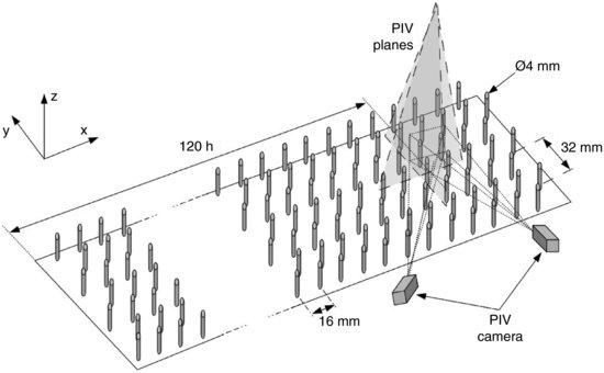
The measurements were performed 120h downstream the start of the vegetation canopy model. At this location, the obtained flow is representative of the flow developing over a vegetation canopy (see Section 11.3.2 for a comparison of the main statistics obtained in the present work with the literature), free from the effect of the change of roughness between the initial fetch of cubes used to generate an urban-like boundary layer and the canopy model. Indeed, in the present case, the canopy drag length scale Lc defined by Belcher et al. (2003) as being characteristic of the length of the adjustment region for the mean flow, is estimated as Lc = 2.6h. In addition, Dupont and Brunet (2009) showed in their study of a canopy edge flow that the adjustment region existing downstream the edge of a canopy has a length of 10h, supporting the fact that the fetch of 120h retained in the present study is sufficient for the flow to be free of the influence of the change of roughness elements.

11.2.3 Stereoscopic PIV setup

In the following, x, y and z denote the longitudinal, spanwise and vertical directions, respectively (Figure 11.1), and u, v, w or u1, u2, u3, the longitudinal, spanwise and vertical velocity components, respectively. Measurements of the instantaneous three-component velocity were performed via stereoscopic particle image velocimetry independently in two different vertical planes: a streamwise aligned (x−z) plane and a spanwise aligned (y−z) plane (Figure 11.1). The laser was arranged so that the light sheet fell in the middle between two cylinder rows. The flow was seeded just at the outlet of the contraction of the wind-tunnel with glycol/water droplets (typical size: 1 μm) using a fog generator. A double-pulsed Litron DualPower 200-15 Nd:YAG laser (wavelength of 532 nm) was used to illuminate the flow. A sampling frequency of 4 Hz was retained to ensure that velocity samples were separated in time by approximately an integral time scale (estimated between 0.15 s and 0.25 s based on the thickness of the boundary layer δ and the mean velocity near the canopy). In each plane, 4000 pairs of images were recorded in order to obtain good convergence of second order statistics (relative error of the velocity variances below 2.5%). In order to measure the three components of the velocity, two Dantec Dynamics FlowSense 4M cameras were mounted in a stereoscopic configuration with an angle about 50° between the camera axis and the normal to the light sheet. These cameras have a resolution of 2048 × 2048 pixels and were equipped with a Nikon AF DC NIKKOR 105 mm f/2D lens. The cameras and the laser were mounted outside the wind tunnel, on the side and above the ceiling, respectively. The Scheimpflug condition was satisfied by rotating the image plane with respect to the lens plane. To ensure this condition, the cameras were installed on special remote controlled mounts designed to enable rotation between the lens and the CCD chip. Image pairs were recorded independently in each plane and processed with an adaptive multi-pass cross-correlation algorithm using 32 × 32 pixels final interrogation windows and a 50% overlap. The dimensions of the obtained velocity fields are approximately with a spatial resolution of 2.66 mm and 1.85 mm in the horizontal and vertical directions, respectively. Given the retained optical arrangement, measurements were performed only above the canopy (1<z/h<5).

11.3 Results

11.3.1 Analysis of instantaneous velocity fields

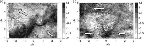
Examples of instantaneous velocity fields (average flow field subtracted) obtained in the longitudinal and transverse planes are shown in Figure 11.2a and b, respectively. Besides ejection and sweep events (grey arrows in Figure 11.2a) that are already known to dominate the momentum transfer in boundary-layer flows (Finnigan, 2000), instantaneous velocity fields exhibit other type of coherent motions. The transverse component v indeed shows the presence of coherent structures in the longitudinal plane that leave a strong imprint on the spanwise velocity (dark colour contour in Figure 11.2a). They appear in the form of regions of nearly constant spanwise velocity, inclined upward with an angle consistent with that of the ejections. In the transverse plane, large regions of constant transverse velocity, elongated in the spanwise direction, are also present (large white arrows in Figure 11.2b). One can notice converging regions of opposite spanwise velocity, merging into an inclined ejection of fluid. This convergence is accompanied by the formation of a lateral shear layer. Small-scale vortical structures appear both at the edge of those constant transverse velocity regions and in the lateral shear layer created near the ejection (thin white arrows in Figure 11.2b).

Figure 11.2 Examples of instantaneous velocity fields (averaged flow field subtracted) measured in (a) the longitudinal plane (vectors: , components) and (b) the transversal plane (vectors: , components), (color contours: component normal to the measurement plane).

11.3.2 One-point statistics

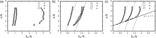
Statistics of the three components of the velocity were computed from the PIV velocity fields obtained in both the longitudinal and the transversal planes by ensemble averaging the data both in time and in the horizontal direction, thus improving the statistical convergence. The cylinder arrangements being periodic, all the statistics were indeed found to be independent of the spanwise or the longitudinal location and the longitudinal growth of the flow due to the natural thickening of the boundary-layer was found negligible (not shown here). This ensemble averaging operation is denoted and denotes the fluctuating part of the ith velocity component.

It must be noted here that the extent of the SPIV measurement domain does not allow for the estimation of the boundary-layer thickness δ. However, from previous preliminary hotwire measurements, δ is estimated to be about 15h. Figure 11.3 shows the main statistics of the flow above the vegetation canopy and their comparison to the data from the experimental study from Brunet et al. (1994) and the numerical one of Finnigan et al. (2009), in similar configurations. First, one can notice that, given the scatter between the different results from the literature (Finnigan, 2000), the present results are found to be in agreement with the two reference cases. The good agreement between the measurements obtained in both planes also confirms the accuracy of the PIV measurements. The Reynolds shear stress is found to be maximal and nearly constant in the region 1<z/h<2 (Figure 11.3c), which allows us to compute the friction velocity in this region (Brunet et al., 1994; Finnigan, 2000). In the present case, 0.615 m/s. This leads to a roughness Reynolds number 2.103 (where is the kinematic viscosity), high enough to ensure that the flow regime is dynamically fully rough. The displacement height d and the roughness length z0 have been estimated by fitting a straight line to the mean longitudinal velocity profile in semi-logarithmic coordinates in the inertial layer. In this region, the mean longitudinal velocity is indeed expected to follow a logarithmic law as where is the von Kármán constant. In the inertial layer of the neutrally stratified atmosphere, the flow is supposed to have a logarithmic mean wind profile but also show a constant correlation coefficient 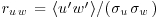, according to the Monin–Obukov similarity theory (Kaimal and Finnigan, 1994). This feature has been confirmed in flow over plant canopies by different in situ and wind tunnel studies (Brunet et al., 1994; Kaimal and Finnigan, 1994; Raupach et al., 1996) which also showed that the magnitude of ruw increases in the roughness sublayer (typically extending from z = h to about 2h). This characteristic behaviour of ruw has been observed in the present study and employed to identify the region of the flow where a similarity theory is valid (2.7<z/h<4.1). The fitting procedure leads to d/h = 0.79 and z0/h = 0.12 for 2.7<z/h<4.1 with .

Figure 11.3 Comparison of present (a) mean and (b) standard deviation of the three velocity components (filled symbols: longitudinal plane, open symbols: transversal plane, circles: u, triangles: v, squares: w) and (c) Reynolds shear stress to (dashed line) the LES from Finnigan et al. (2009) and (solid line) the experiment from Brunet et al. (1994).

The quantity is found to be equal to nearly zero, confirming the assumption that the flow is statistically homogeneous in the spanwise direction (not shown here).

Figure 11.3b shows the vertical evolution of the standard deviation of each component. The standard deviation of the longitudinal and transversal components are nearly constant in the regions 1.5<z/h<2.1 and 1.7<z/h<2.8, respectively, whereas does not exhibit any plateau. Moreover, as expected, the longitudinal component u is the largest contributor and, surprisingly but in agreement with what can be observed in the instantaneous velocity fields, the spanwise component v contributes to more than 25% to the turbulent kinetic energy, actually more than the vertical component w (Figure 11.3b, open triangles). This high level of fluctuation, associated to a strong spatial coherence observed in the instantaneous velocity fields (Figure 11.2) is believed to be the footprint of coherent structures from the boundary-layer interacting with the canopy.

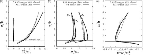
Figure 11.4a shows the evolution of the skewness of the three velocity components defined as . The skewness Sv of the transversal velocity component is found to be equal to zero, again supporting the assumption of statistical homogeneity of the flow in the spanwise direction. In agreement with the literature, Su is found to be positive for z/h<3, corresponding to a predominance of high-speed events near the canopy and a predominance of low-speed events above.Sw is found to be negative for z/h<2.2 and positive above. By using the quadrant-hole technique, one can perform a conditional analysis of the velocity fields in order to determine the number of ejection (or Q2) and sweep (or Q4) events (defined here as and and and , respectively) that are known to be responsible for momentum transfer in boundary-layer flows (Finnigan, 2000). Figure 11.4b shows the vertical distribution of the number of ejections and sweeps detected in the present dataset. Accordingly to the previous analysis of the velocity skewness, more sweeps (Q4) than ejections (Q2) occur near the canopy. This tendency reverses for z/h>3.

Figure 11.4 Evolution with the distance to the canopy of (a) the skewness of the velocity components (: u, : v, : w) and (b) the number of Q2 and Q4 events.

11.3.3 Two-point statistics

In this section, in order to assess the structure of the coherent turbulent motion, an analysis of the evolution of the two-point correlation coefficient 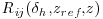is presented. Rij is defined as:

(11.1)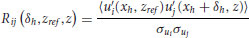

where xh denotes the horizontal direction in the considered plane (e.g xh = x in the longitudinal plane or xh = y in the transversal plane) and the spatial separation of the two points in the horizontal direction. Again, ensemble averaging is performed both in time and in the horizontal direction (x or y). For the sake of brevity, two-point correlation coefficients of the longitudinal and vertical components in the longitudinal plane are not presented here as they exhibit shapes and levels in agreement with the organization of turbulent boundary-layer flows proposed in the literature that corresponds to packets of hairpin vortices (Adrian, 2007).

The focus is here on the spanwise component and its spatial structure, as very little information about it has been reported in previous studies. In the longitudinal plane (Figure 11.5a, c), Rvv shows an elongated structure of elliptical shape, the major axis of which being tilted with an angle of 30° against the horizontal plane. It is noticeable that, due to the inclination, the typical length scale of the major axis is in fact longer than the longitudinal length scale associated to this correlation coefficient. Regions of low-level negative correlation can be seen below and downstream and above and upstream the reference point. Near the canopy (Figure 11.5c), the shape of the correlation is clearly affected by the presence of the canopy. In the transversal plane (Figure 11.5b, d), the correlation function also exhibits an elliptical shape, the length scales of which grow with the distance to the canopy. Near the canopy (Figure 11.5d), long-range low levels of correlation and also negative correlation with the flow above exist.

Figure 11.5 Two-point correlation coefficients of the transversal component Rvv in (a, c) the x−z plane and (b, d) the y−z plane obtained at (a, b) zref/h = 3.4 and (c, d) zref/h = 1.2. Positive contours: white, negative contours: black, contour increment: 0.1, black solid line: zero-contour.

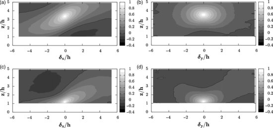
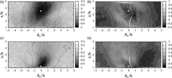
Cross-correlations Rvu and Rvw in the transversal plane of the spanwise component with the other components u and w (Figure 11.6) show regions of positive and negative correlation located on each side of the reference point. It reveals that v is strongly correlated with high and low speed regions (Figure 11.6a, c) and downward and upward regions (Figure 11.6b, d), in agreement with the existence of ejection and sweep events in a turbulent boundary-layer (Finnigan, 2000; Adrian, 2007). Again, near the canopy, the correlation patterns exhibit long-range correlation with the flow above, reinforcing the fact that a strong interaction exists between the turbulent boundary-layer and the region near the canopy. If the reference point is high enough above the canopy (z/h>3.1), regions of positive and negative correlation appear below the reference point (Figure 11.6a, b).

Figure 11.6 Two-point cross-correlation coefficients in the y−z plane: (a, c) Rvu and (b, d) Rvw obtained at (a, b) zref/h = 3.4 and (c, d) zref/h = 1.2 (white square). Positive contours: white, negative contours: black, contour increment: 0.1, black solid line: zero-contour.

11.3.4 Length scales of turbulent structures

The computation of the two-point correlation coefficients described above allows for the estimation of the integral length scales for the three components, in the three directions. These integral length scales provide an estimate of the size of the large energy-containing turbulent structures and the analysis of their evolution across the boundary layer enables the identification of self-similar structures (Tomkins and Adrian, 2003).

The integral length scale associated to the velocity uj in the direction xi is usually defined as 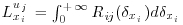where is the spatial separation between the two points in the direction xi (Kaimal and Finnigan, 1994). In most of the cases, integrating the correlation coefficient is not feasible. An alternative approach is to approximate by an exponential function of . In this case, the integral length scale can be computed directly and is given by the value of where reaches the level of (Kaimal and Finnigan, 1994). In the present work, the value of 1/e is rounded up to 0.4. is thus defined as the distance from the reference point (maximum of correlation) to the point where the correlation coefficient reaches the value of 0.4 in that direction. It must be noted here that the vertical integral length scales are defined in the direction from the reference point down to the canopy. Results are presented in Figure 11.7. It is worth noting here that, in these plots, all the dashed lines have the same slope. Concerning the longitudinal integral length scales of the longitudinal and vertical components (Figure 11.7a), a good agreement with Finnigan (2000) is found, despite a slight underestimation, probably due to the use of a threshold of 0.4 instead of the complete spatial integration of the correlation function. Qualitatively, it can be seen that almost all the integral length scales grow linearly with the distance to the canopy with changes of slope for certain length scales. Strikingly, the three length scales LuZ, LvZ and LwZ show the same growth rate in different regions (Figure 11.7c). Moreover, just above the canopy, the vertical length scale LuZ is directly given by the distance to the canopy (it follows the line z/h = Luz+1) and seems tightly linked to LvZ. Above z/h = 3, its growth rate decreases. Interestingly, LvZ follows the same trend but the influence of the canopy on its growth rate is limited to the region below z/h = 1.75

Figure 11.7 Evolution with the distance to the canopy of the length scales in (a) the longitudinal direction, (b) the transversal direction and (c) the vertical direction (: u, : v, : w)

Several length scales are shown to vary linearly with distance from the wall, revealing self-similar growth of structure in an average sense (Tomkins and Adrian, 2003) and the analysis of their growth rate gives some information on the spatial structure of this coherent eddies. Low and high speed regions are thus tightly linked to a coherent spanwise motion that statistically takes place below, which is supported by the existence of maxima of correlation Rvu above and on each side of the reference point (Figure 11.6a, c). The fact that the growth rates of the vertical length scales of these two structures are linked supports the conclusion that spanwise and longitudinal coherent motions are part of the same coherent structure. In addition, the canopy has a strong influence on the structure of the flow in the region 1<z/h<3, which can be interpreted as the existence of an attached (close to the canopy) and a detached regime (beyond z/h = 3, which roughly corresponds to the bottom of the inertial layer).

11.3.5 Qualitative evidence of very-large scale structures

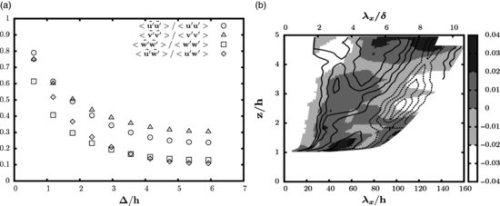
In the present study, in order to go further in the analysis of the spanwise component and its relationships to the coherent motions existing in the flow over vegetation canopies, the same procedure as Inagaki and Kanda (2010) was employed. Their method is based on the use of a spanwise filter designed to investigate the existence of a bimodal behaviour of the velocity in the horizontal plane. This analysis was performed in the transversal plane (y–z) and a moving average filter of half-width was used to filter out the high frequency mode from the three velocity components and retain the low frequency part, defined as:

(11.2)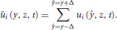

The effect of the half-width on the statistics of the low frequency part is presented in Figure 11.8a (shown for z/h = 1.5). It can be seen that as is increased, the ratio between over of the unfiltered values decreases as more and more fluctuations are removed from the signal. As reported by Inagaki and Kanda (2010), this ratio decreases faster when the vertical component and the shear-stress are considered. This is consistent with the above analysis of integral length scales and with the fact that very large-scale motions consist of superstructures meandering in the horizontal plane and that vertical motions related to ejections and sweeps are events of smaller scales. When , the filtered horizontal components and account for 30% of the unfiltered turbulent intensities whereas the filtered and represent less than 15% of the unfiltered values. Following the original hypothesis of Townsend (1976) and the recent study of Inagaki and Kanda (2010) who defined the active part (of high-frequency mode) of the fluctuations as being the largest contributor to the shear-stress and vertical fluctuations, the filter width is set here to , the maximum value that allows for the minimum values of and relative to the unfiltered values.

Figure 11.8 (a) Evolution of the ratio of the turbulent intensities filtered in the spanwise direction and unfiltered for different sizes of filter at z/h = 1.5. (b) Temporal correlation of the large-scale motion as a function of the distance to the canopy (line contours: with negative levels: dashed lines, positive levels: solid lines, colour contours: ).

An attempt to further characterize, at least qualitatively, the low-frequency mode is presented here, by using the fact that SPIV velocity fields were recorded at the frequency of 4 Hz. This frequency of acquisition is too low to resolve most of the turbulence spectrum but is able to capture the low frequency fluctuations associated to the superstructures that may exist in the present flow. Recent studies focusing on very large-scale structures over smooth wall (Hutchins and Marusic, 2007; Lee and Sung, 2011) or urban-like terrain (Inagaki and Kanda, 2010) have indeed shown that the length of these structures is of the order of several times δ (up to 20 times, with an average length close to , Hutchins and Marusic, 2007) and are responsible for very low levels of correlation at large separation when considering streamwise two-point correlations. Based on this estimation of the size of the very-large scale structures, time correlations from acquisitions performed at 4 Hz as in the present study are likely to miss the smaller structures the size of which below but detect the presence of longer structures, which leave a small imprint in the temporal correlations.

If meandering superstructures do exist in the present flow, they are expected to leave their imprint on the long-range temporal correlation (or spatial correlation in the streamwise direction) as alternating positive and negative correlation levels, with a large wavelength. Obviously, the limited acquisition frequency will prevent us from obtaining an accurate estimate of a particular wavelength. In order to reduce the influence of the small-scales, the 4000 velocity fields recorded in the normal plane were first filtered using the above defined spanwise moving average filter () and then used to compute temporal correlation coefficients defined as:

(11.3)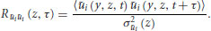

The local mean longitudinal velocity is then used to recover the streamwise spatial separation, using the Taylor's frozen turbulence hypothesis. The obtained correlation and are shown superimposed in Figure 11.8b (line contours: , color contours: ). Correlation levels are very low (below 0.05 in magnitude) but are comparable to those reported by Hutchins and Marusic (2007). This can be explained by the fact that the superstructures are unlikely to be of purely sinusoidal shape in the horizontal plane. The jitter of the superstructures is expected to reduce the correlation levels. Despite these low levels, correlation maps clearly exhibit alternation of positive and negative levels, with very large spatial separations that depend on the distance to the canopy. Strikingly, the wavelengths associated with the longitudinal and the transverse components are very similar, supporting the fact these correlation patterns are the footprint of the same large-scale elongated structures existing in the horizontal plane. The typical longitudinal length scales that can be extracted from these correlations are of the order of several times the height of the boundary-layer and consistent with those reported by Hutchins and Marusic (2007) and Inagaki and Kanda (2010). However, because of the very low acquisition frequency, the accuracy in the time domain is low and the quantitative analysis and characterization of the detected superstructures remain open. (not shown here) does not exhibit any particular very large-scale organization, in agreement with the fact that vertical motions are more compact in the longitudinal direction.

11.3.6 Conditional averaged velocity fields

In order to further investigate the relationships between the spanwise component and the sweep and ejection events, conditional averaged velocity fields were computed in the spanwise-wall normal plane by averaging the velocity fields corresponding to the simultaneous occurrence of an ejection (or a sweep) event together with a positive spanwise velocity. The goal here is to take into account the fact that ejections and sweeps that are primarily responsible for momentum transfers in the flow over a vegetation canopy are in fact embedded in elongated superstructures that meander in the horizontal plane and are therefore animated by a fluctuating transverse motion.

Due to the statistical spanwise homogeneity of the flow, results obtained for a negative spanwise velocity are nearly identical, the only difference being that one is the symmetric of the other. Moreover, to select strong ejection or sweep events, a threshold has been imposed on the fluctuating velocity at the reference point. The conclusions drawn from the present analysis do not differ if this threshold is set to zero. The condition chosen to compute the conditional average then reads:

(11.4)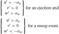

Figure 11.9a, c shows the results obtained in the case of an ejection event, at two different heights above the canopy. The conditional velocity fields are consistent with the occurrence of an ejection at the reference point, characterized by a low-speed upward motion. One can notice that the low momentum region is systematically flanked by a high-speed downward motion, in agreement with the turbulent structure of boundary-layer flows. However, imposing a positive spanwise velocity breaks the symmetry of the structure usually found in the literature and reveals that there exists a spanwise motion from the high-speed to the low-speed region. This is confirmed by the computation of the conditional average velocity field given the occurrence of a sweep event (Figure 11.9b, d). The analysis of the results obtained close to the canopy (Figure 11.9c, d) shows that there is a preferred organization corresponding to a region of high-speed downward flow located on the left side of the ejection, in the case of a positive spanwise velocity at the reference point. These two regions are linked by a spanwise motion, located below the reference point. These conditional average velocity fields also show the presence, between the low and high momentum regions, of large-scale vortical motions of streamwise axis, the scale of which is larger than the vortical structures that were observed in the instantaneous velocity fields (Figure 11.2). These streamwise vortical structures are believed to be an artefact of the averaging process and reflect the contribution to the ensemble-averaged velocity field of structures composed of an inclined sweep with a spanwise motion below or an inclined sweep with a spanwise motion above but oriented in the opposite direction. The combination of these types of structures is indeed more in agreement with the analysis of the instantaneous flow fields in which large-scale streamwise vortices were not to be seen.

Figure 11.9 Conditional average velocity field obtained for (a, c) an ejection or (b, d) a sweep event combined to a positive spanwise velocity occurring at (white square) (a, b) zref/h = 3.4 and (c, d) zref/h = 1.2 (one every three vector is shown for clarity).

11.4 Discussion and conclusion

The present study focuses on the turbulent flow developing over a vegetation canopy, and on its spatio-temporal organization. Measurement of the three velocity components in both a longitudinal and normal planes allows us to gain further insight into the contribution of the spanwise component to the turbulent structures that are already known to exist in boundary-layer type flows, namely ejections and sweeps located in low- and high-speed regions, respectively. Even if the effect of the spanwise component often disappears from the balance equations due to the commonly made assumption of statistical spanwise homogeneity, it has been shown here that this component exhibits high levels of fluctuation and plays an important role in the unsteady dynamics of the flow by providing a link from high to low momentum regions.

The findings of this chapter are summarized in the sketch shown in Figure 11.10 and are discussed in the following. Analysis of the two-point correlations in the x–z plane showed that the spanwise fluctuations organize themselves in coherent structures that are elongated in the longitudinal direction and inclined upward with an angle close to 30° (Figure 11.5a, c). This inclination angle is very close to the inclination angle of hairpin vortices (between 30° and 60°) reported by Adrian (2007), and larger than the inclination of the low-momentum they measured (12°). Hence, it is likely that the coherent spanwise motion detected in this plane is strongly related to hairpin-like structures. The flow being homogeneous in the spanwise direction, no further information could be extracted from this plane. Analysis of the statistics in the y–z plane showed that this inclined structure is also elongated in the spanwise direction with an extent of the same order as the distance between ejection and sweep events that can be deduced from the correlation Ruw in this plane (Figure 11.5b, d). Cross-correlations Rvu and Rvw showed that this coherent spanwise motion (dark grey arrows in Figure 11.10) is preferentially found under and between an ejection and a sweep (labelled Q2 and Q4 in Figure 11.10) when the considered reference point is close to the canopy (Figure 11.6c, d), and above or below (with the same level of correlation) when the reference point is far enough from the top of the canopy (Figure 11.6a, b). In agreement with the continuity of the velocity field, the spanwise motion always goes from the sweep to the ejection. Cross-correlations Ruv and Rwv (not shown here) confirm this spatial organization.

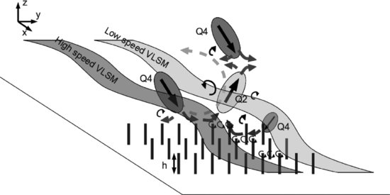
Figure 11.10 Sketch summarizing the spatio-temporal dynamics of the flow above a vegetation canopy showing high- and low-speed meandering superstructures in which sweeps (Q4) and ejections (Q2) linked by spanwise motion (thick dark grey arrows) and generating large-scale rotating motion (light grey dashed arrows) and small-scale vortical structures between them and near the canopy (thin black arrows).

Stanislas et al. (2008) demonstrated that hairpin vortices are statistically more likely to be nonsymmetric one-legged canes than perfectly symmetric two-legged arch. Based on this, a conditional analysis of the velocity field was performed on the occurrence of an ejection or a sweep event. A positive (left-to-right) spanwise motion was also imposed in the condition at the reference point to break the statistical symmetry. Conditional averages in Figure 11.9 confirm that an ejection is flanked by a sweep (laterally inclined Q2 and Q4 in Figure 11.10), the two being linked by a spanwise motion occurring below. Close to the canopy (Figure 11.9a, b), the condition of positive spanwise velocity leads preferentially to the occurrence of a sweep on the left side of an ejection. When the reference point is further from the canopy (Figure 11.9c, d), in the case of an ejection (sweep), converging (diverging) spanwise flows are observed on both sides. This organization gives rise to large-scale vortical motions of streamwise axis (light grey dashed arrows in Figure 11.10) and leaves the same statistical imprint as the large-scale streamwise vortical structures that were reported in previous studies based on the use of empirical orthogonal functions (EOF) (Finnigan and Shaw, 2000). This technique, based on the decomposition of the two-point correlation tensor becomes equivalent to the Fourier transform when performed in a homogeneous direction (Berkooz et al., 1993). Spanwise modes can only be symmetric or antisymmetric with respect to the vertical direction, as the flow is statistically homogeneous. As noted by Finnigan et al. (2009), the EOF-derived structure is the ensemble average of hairpin vortices. From the present analysis, the instantaneous structures are more likely to be composed of inclined ejections or sweeps with spanwise fluid motion above or below, linking high- and low-speed regions, inclined upward in the same manner as the hairpin structures (see example in Figure 11.2).

Analysis of typical length scales in the vertical direction of the coherent structures extracted from the two-point correlations supports the fact that the extracted coherent motions in the three directions are part of the same coherent structure as they have the same growth rate (Figure 11.7). The presence of a region of influence of the canopy that extends, in the present case, over 2h above the canopy has also been shown. This influence can be interpreted as the transition from an attached to a detached regime when moving away from the canopy (Figure 11.7c). The height where the correlation regime switches () corresponds to the location where the skewness of the longitudinal component changes of sign and where the number of detected ejection events becomes larger than the number of sweeps (Figure 11.4). This corresponds also to the bottom of the inertial layer. The coherent structures present below z/h = 3 are likely to strongly interact with the canopy flow and elements, which may explain that the relative importance of ejections and sweeps depends on the distance to the canopy. However, the relationships between these two regimes and their interaction mechanisms remain to be studied.

Besides its important role within hairpin-like structures, the spanwise component has also been found to be involved in inactive superstructures that consist of low- or high-speed regions that meander in the horizontal plane (labelled VLSM in Figure 11.10). The streamwise length scale of these structures is of the order of several times the height of the boundary layer. The presence of these superstructures supports the fact that instantaneous coherent structures are animated by a spanwise motion that alters the symmetric organization that can be inferred from the two-point statistics. Moreover, Hutchins and Marusic (2007) and Hutchins et al. (2011) showed that theses superstructures, in which the hairpin vortices organize in packets (Adrian, 2007), were responsible for modulating near-wall small-scale activity and skin friction events in the case of a smooth wall boundary layer. In the present study, even if the condition at the wall is completely different, one can expect to find an influence of the large-scales over the small-scales, supporting the existence of a top-down mechanism (Drobinski et al., 2004). This is likely to result in a strong interaction between the outer flow and the canopy, with the generation of strong vertical gradient of both the longitudinal and spanwise velocity components and small three-dimensional structures stretched by the high mean shear existing near the top of the canopy (thin black arrows in Figure 11.10).

Finally, even if the one-point statistics of the present flow share some common features with those of a mixing layer (Finnigan, 2000), the comparison of the two-point correlation tensor with the one measured in a canonical mixing layer shows that the spatio-temporal structure of the turbulence is different. In particular, Delville et al. (1999) reported that Kelvin–Helmholtz structures and the associated longitudinal vortices lead to the presence of zero-crossings in the two-point correlation of the three components of the velocity in the longitudinal direction, the position of which scaling with the vorticity thickness. The same comment can be made for the organization in the spanwise direction. These characteristics, typical of a plane mixing layer, have not been noticed in the present correlations, nor in the instantaneous flow fields.

Based on the present findings, further work is needed to investigate the dynamics of the interaction between the structures educed above the canopy and the flow within the canopy itself, the role of inactive large-scale motions on the smaller scales close to the canopy and on the transfer mechanisms between the canopy and the flow above, the spatial organization of the superstructures, among others.

11.5 Acknowledgements

This work was performed in the framework of the project ANR Villes Durables – VEGDUD, funded by the French National Research Agency (ANR) under contract ANR-09-VILL-0007-01.

References

Adrian, R.J. (2007) Hairpin vortex organization in wall turbulence. Physics of Fluids 19, 041301. DOI: 10.1063/1.2717527.

Belcher, S.E., Jerram, N. and Hunt, J.C.R. (2003) Adjustment of a turbulent boundary layer to a canopy of roughness elements. Journal of Fluid Mechanics 673, 255–285.

Berkooz, G., Holmes, P. and Lumley, J.L. (1993) The proper orthogonal decomposition in the analysis of turbulent flows. Annual Review of Fluid Mechanics 25, 539–575.

Brunet, Y., Finnigan, J.J. and Raupach, M.R. (1994) A wind tunnel study of air flow in waving wheat: single-point velocity statistics. Boundary-Layer Meteorology 70, 95–132.

Castillo, M.C., Inagaki, A. and Kanda, M. (2011) The effects of inner- and outer-layer turbulence in a convective boundary layer on the near-neutral inertial sublayer over an urban-like surface. Boundary-Layer Meteorology 140, 453–469.

Cheng, H., Hayden, P., Robins, A.G. and Castro, I.P. (2007) Flow over cube arrays of different packing densities. Journal of Wind Engineering and Industrial Aerodynamics 95, 715–740.

Delville, J., Ukeiley, L., Cordier, L. et al. (1999) Examination of large scale structures in a turbulent plane mixing layer. Part 1: Proper Orthogonal Decomposition. Journal of Fluid Mechanics 391, 91–122.

Drobinski, P., Carlotti, P., Newsom, R.K. et al. (2004) The structure of the near-neutral atmospheric surface layer. Journal of Atmospheric Science 61, 699–714.

Dupont, S., and Brunet, Y. (2009) Coherent structures in canopy edge flow: a large-eddy simulation study. Journal of Fluid Mechanics 630, 93–128.

Finnigan, J.J. (2000) Turbulence in plant canopies. Annual Review of Fluid Mechanics 32, 519–571.

Finnigan, J.J. and Shaw, R.H. (2000) A wind-tunnel study of airflow in waving wheat: an EOF analysis of the structure of the large-eddy motion. Boundary-layer Meteorology 96, 211–255.

Finnigan, J.J., Shaw, R.H. and Patton, E.G. (2009) Turbulence structure over a vegetation canopy. Journal of Fluid Mechanics 637, 387–424.

Hutchins, N. and Marusic, I. (2007) Evidence of very long meandering features in the logarithmic region of turbulent boundary layers. Journal of Fluid Mechanics 579, 1–28.

Hutchins, N., Monty, J.P., Ganapathisubramani, B. et al. (2011) Three-dimensional conditional structure of a high-Reynolds-number turbulent boundary layer. Journal of Fluid Mechanics 673, 255–285.

Inagaki, A. and Kanda, M. (2010) Organized structure of active turbulence over an array of cubes within the logarithmic layer of atmospheric flow. Boundary-Layer Meteorology 135, 209–228.

Kaimal, J.C. and Finnigan, J.J. (1994) Atmospheric Boundary-Layer Flows – Their Structure and Measurement, Oxford University Press, New York.

Lee, J.H. and Sung, H.J. (2011) Very-large-scale motions in a turbulent boundary layer. Journal of Fluid Mechanics 673, 80–120.

Manes, C., Poggi, D. and Ridolfi, I. (2011) Turbulent boundary layers over permeable walls: scaling and near-wall structure. Journal of Fluid Mechanics 687, 141–170.

Poggi, D., Porporato, A., Ridolfi, I. et al. (2004) The effect of vegetation density on canopy sub-layer turbulence. Boundary-Layer Meteorology 111, 565–587.

Raupach, M.R., Finnigan, J.J. and Brunet Y. (1996) Coherent eddies and turbulence in vegetation canopies: the mixing-layer analogy. Boundary-Layer Meteorology 78, 351–382.

Stanislas, M., Perret, L. and Foucaut, J.M. (2008) Vortical structures in the turbulent boundary layer: a possible route to a universal representation. Journal of Fluid Mechanics 602, 327–387.

Tomkins, C.D. and Adrian, R.J. (2003) Spanwise structure and scale growth in turbulent boundary layers. Journal of Fluid Mechanics 490, 37–74.

Townsend, A.A. (1976) The Structure of Turbulent Shear Flow, Cambridge University Press, Cambridge.