12
Calculation and Eduction of Coherent Flow Structures in Open-Channel Flow Using Large-Eddy Simulations
ABSTRACT
In this chapter, an introduction is given to the large eddy simulation (LES) technique applied to open-channel flows, together with examples in which LES was employed to reveal the generation and fate of coherent flow structures. A brief description of the fundamentals of LES is provided, mainly regarding how large-scale and small-scale motions of turbulence are separated, showing that while the large scales are solved directly, the small-scale motions require some sort of modeling. Three application examples are presented, including straight open channel flow over smooth, rough and permeable beds, flow through emergent vegetation and flow over dunes. These examples demonstrate the enormous potential of LES to investigate coherent flow structures. In addition, the present capabilities and future potential of LES for geophysical flow calculations are highlighted and discussed.
12.1 Introduction
The flow in open-channels features a large variety of coherent turbulent structures, many of which result from shear layer turbulence generated near the channel bed or as a result of channel planform or bed topology, such as channel expansions, pool-riffle sequences or bedforms. Other coherent structures are generated from the interaction of the flow with man-made hydraulic structures, for instance groynes, bridge piers, or due to large-scale roughness elements such as boulders, vegetation or debris, in which the flow separates and large-scale flow structures develop as a result of local flow separation, recirculation, shear layer formation and vortex shedding.
In geophysical alluvial flows, there is the need to understand the generation and behaviour of coherent flow structures, because they are mainly responsible for the transport of sediments and solutes, and are hence vital in determining channel morphology and evolution of the fluvial landscape. Coherent structures have been the subject of many experimental studies (e.g. the pioneering work by Kline et al., 1967; Corino and Brodkey, 1969; Grass, 1971; Willmarth and Lu, 1972) and have been identified in these early works on boundary layer turbulence mainly through visualization or conditional sampling techniques. Although no clear definition of ‘coherent structures’ exists, it is commonly agreed that a coherent structure is a region of space (or time) within which the flow field has a characteristic coherent flow pattern (Pope, 2000). In his review article, Robinson (1991) provides the following definition: ‘a three-dimensional region of the flow over which at least one flow fundamental variable exhibits significant correlation with itself or with another variable over a range of space and/or time that is significantly larger than the smallest scale of the flow’. Nezu and Nakagawa (1993) introduce and discuss coherent structures in the context of open-channel flows and distinguish between ‘bursting-structures’ near the channel bed and ‘large-scale vortical structures’ that are generated by the mean flow and/or the channel geometry away from the bed. In Table 12.1, which builds upon the categorization according to Robinson (1991), the most common coherent flow structures/events occurring in open-channel flows are summarized. The first five structures are considered ‘bursting-structures’ or ‘bursting-events’, whereas the last seven are categorized as ‘large-scale vortical structures’.
Table 12.1 Coherent structures found in turbulent flows in open channels.
| Structure | Description |
| Low- and high-speed streaks | Elongated areas of alternating high- and low-speed fluid |
| Burst event | Lift-up and bursting of low-speed streaks including sweeps and ejections |
| Ejection event | Ejection of low momentum fluid away from the wall |
| Sweep event | Inrush of high momentum fluid from outer layer |
| Hairpin vortices | Near-wall spanwise vortices with elongated trailing legs |
| Horizontal/vertical rollers | Vortices with distinct rotation about a one-dimensional axis |
| Horseshoe vortices | Vortices as a result of three-dimensional boundary layer separation due to flow obstruction |
| Von Kármán type vortices | Shear layer roll-up and shedding of vortices into the wake behind bluff bodies |
| Kelvin–Helmholtz instabilities | Internal instabilities as a result of strong velocity shear |
| Tornado vortices | Funnel-shaped vertical axis vortices |
| Shear layer backs | Sloping streamwise velocity discontinuities |
| Boils, Kolk-boils | Strong upward vortex motion initiated near the bed |
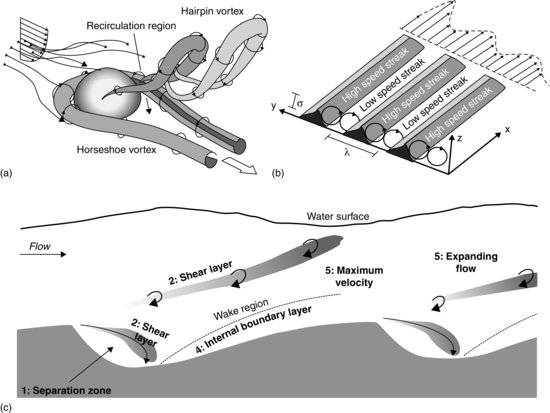
An enormous amount of experimental research has been dedicated since the above pioneering work within the geophysical and hydraulic communities in order to detect, analyse and quantify coherent structures and their effect on the statistics of the flow and the transport of mass and momentum (for instance associated with dunes, vegetation or rough beds). Great progress has been made in developing an understanding of coherent flow structures, which has led to a number of conceptual models for diverse types of structures. Figure 12.1 depicts three conceptual models of turbulent coherent flow structures in open-channel flow: (a) over a roughness element, as suggested by Bezzola (2002), (b) over a smooth wall, and (c) over dunes, as proposed by Best (2005).
Figure 12.1 Conceptual models of (a) coherent structures in flow over a roughness element (after Bezzola, 2002 (and adapted from Acarlar and Smith, 1987). Reproduced with permission from Cambridge University Press) (b) near-wall streaks in flow over a smooth wall; (c) flow over dunes (reproduced from Best, 2005. Copyright © 2005 American Geophysical Union, with permission from John Wiley & Sons).
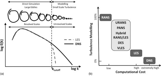
Contributions to advance knowledge on coherent flow structures in channel flow from numerical simulations have been limited until recently. This is mainly because most simulations to date have been carried out with so-called Reynolds-averaged Navier–Stokes (RANS) methods, in which the time-averaged equations for mean-flow quantities are solved, i.e. the turbulence is averaged out and its effect is accounted for entirely by a turbulence model. Although RANS methods are economical and can predict the mean flow at any spatial scale, flow unsteadiness and turbulence (i.e. coherent flow structures) and resulting unsteady forces on the channel bed and in-stream obstacles and structures cannot be resolved by RANS models. The advent of supercomputers in the early 1980s enabled direct numerical simulations (DNS), a method in which the exact 3D, time-dependent, Navier-Stokes equations are solved numerically without any model, thereby resolving all scales of turbulent motion from the large eddies down to the smallest, dissipative scales. To date, DNS of relatively low Reynolds number channel flow have enabled researchers to educe and quantify three-dimensional coherent structures, such as streaks and hairpin vortices, that prevail in channel flow over a smooth wall (e.g. Kim et al., 1987; Kim, 1989; del Álamo and Jiménez, 2003; Jiménez et al., 2004). However, as the size of the smallest scales relative to the extent of the flow domain decreases linearly with the Reynolds number (Re), the number of grid points necessary for resolving all motions in a 3D calculation increases roughly with Re3. As a consequence, for Reynolds numbers of practical relevance in geophysical flows, the number of grid points required becomes so large that the computational effort exceeds by far the capabilities of even the biggest available computers. The method of large-eddy simulation (LES) lies in between RANS and DNS, both in terms of numerical effort and its need for modelling turbulence (Figure 12.2b). Like DNS, LES also solves the 3D time-dependent flow equations, but only large-scale, energetic turbulent motions are resolved both in time and in space, and the effects of smaller scales on the large ones are modelled (this is conceptually sketched Figure 12.2a). More details of LES are given below. LES offers a substantial increase in accuracy over time-averaged approaches, particularly when large-scale turbulent structures dominate the flow and the related processes of mass and momentum transfer (Rogallo and Moin, 1984).
Figure 12.2 (a) Illustration of the concept of LES and (b) LES versus RANS versus DNS versus other approaches in terms of computational effort and amount of turbulence modelling.
In recent years, a number of large-eddy simulations have been performed to complement existing laboratory experiments. Often, the data from an experiment are used to validate the simulation, which in turn provides all flow quantities at every instant in time and at every location in the flow. This is particularly significant for quantities that are very difficult to measure, such as pressure fluctuations, or at locations in the flow where measurements are impossible, such as very close to the wall. According to Keylock et al. (2005), LES promises to become an important research tool in the simulation of sediment transport and fluvial processes, especially when considering the fact that coherent turbulent structures are mainly responsible for the entrainment of sediment into suspension and their transport by turbulent dispersion (Sutherland, 1967; Nino and Garcia, 1996; Nezu et al., 1997) or for the incipient motion of bedload transport (Müller and Gyr, 1996). In this chapter, the method of LES is introduced briefly and common features, strengths and weaknesses are discussed. Three examples are then presented in which LES was employed to investigate coherent flow structures in geophysical open-channel flows.
12.2 Method of LES
The concept of LES is to simulate directly (resolve) the large-scale structures (large eddies) that are generated by the geometry and boundaries, and are therefore unique to the problem at hand. The smaller eddies are more universal, and their effect on the large-scale motion is unresolved by the numerical method and can be specified by a model that contains a small number of nearly universal parameters (Rogallo and Moin, 1984; Ferziger, 1996; Lesieur and Metais, 1996). The governing equations for the fluid flow are the filtered incompressible Navier-Stokes equations for the resolved velocity and the resolved pressure (e.g. Sagaut, 2003):
(12.1) 
(12.2) 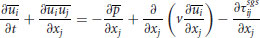
where  and
and  (i or j = 1, 2, or 3) are the resolved velocity vectors and
  is the resolved pressure divided by the density. These quantities are usually filtered in space (indicated by the overbar); more information on the filtering process is given below. Similarly, xi and xj represent the spatial location vectors,
  is the kinematic viscosity and the
  term is the unresolved subgrid-scale fluctuations. The
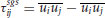
  term represents the effect of the unresolved turbulent fluctuations on the resolved flow, and since it acts like a stress and cannot be computed explicitly it needs to be approximated by a so-called subgrid scale (SGS) model. Similar to the RANS community, there are a number of different approaches to model the SGS stresses, introduction and discussion of which are omitted for brevity herein but can be found in the standard LES literature (e.g. Rogallo and Moin, 1984; Ferziger, 1996; Sagaut, 2003). The filtering procedure separates the turbulent motion into large scales and small scales, which, when examined in an idealized sense, are quite distinct (Table 12.2) from each other. From Table 12.2, it is obvious why LES, when executed correctly, has had such success in simulating accurately flows that are dominated by large-scale motions, because the energetic portion of the flow is resolved. The filtering is theoretically straightforward, and the local quantities are split into a resolved part and deviations from these (i.e. the subfilter fluctuations), for which formal filter functions can be applied (e.g. Sagaut, 2003). However, applying such filter functions formally and in an explicit way is not very common because in such spatially well-resolved simulations (as in LES) the numerical grid can be used as a (spatial) filter. The distance between two-grid points equals the filter width, and hence the quantities that are calculated at a grid point are the turbulent motions that can be resolved (by the given grid), with small-scale fluctuations (in a spatial sense) that cannot be resolved falling through the chosen grid. These fluctuations as formulated in Equation (12.3) are thus called subgrid stresses, rather than subfilter stresses. In LES, the primary goal of an SGS-model is to dissipate the correct amount of energy from the directly calculated large-scale flow, and to allow for a physically realistic exchange of energy between the resolved scales. The most important interactions to be modelled by the SGS model are those between the largest unresolved (subgrid) scales and the smallest resolved scales. In a well resolved LES, the boundary between the resolved (larger) and unresolved (smaller) scales is situated within the inertial subrange, and this boundary is often referred to as the cut-off wave number (dashed line in Figure 12.2a). The concept of LES is illustrated in an idealized way in Figure 12.2a by using the Kolmogorov diagram. The energy spectra of the flow as simulated by a DNS (solid line) and a LES (dashed line) are plotted. Ideally, the spectra in the production range and in the larger part of the inertial subrange are identical, indicating that both LES and DNS simulate directly the large-scale motions. In LES, the transfer of energy from the large scales to the small scales is aided by the SGS model. At smaller scales, the dissipative virtue of the SGS model is visible, particularly in the vicinity of the cutoff wave number (kcutoff). Beyond this wave number, the SGS model causes much faster energy dissipation in the LES than in the DNS. In implicitly filtered LES, the cutoff wave number is determined by the grid, which in most simulations is dictated by the available computational resources. The finer the grid, and thus the more of the spectrum that can be resolved, the less important the SGS model. Hence, the success of an LES depends to a great deal on the chosen grid resolution.
Table 12.2 Large and small-scales of turbulent channel flow.
| Large scales | Small scales |
| Generated from the mean flow | Generated from the large scales |
| Dependent on boundary conditions and specific flow geometry | Universal |
| Show structures | Unorganized |
| Inhomogeneous and anisotropic | More homogeneous and less anisotropic |
| Energetic | Less energetic |
| Diffusive | Dissipative |
 Very difficult to model Very difficult to model
|
 Easier to model Easier to model
|
The method of LES evolved as a computationally less demanding alternative to DNS in the early 1970s but, as mentioned above, the energetic part of the spectra is, ideally, still resolved directly by the numerical method. Hence, and as illustrated in Figure 12.2b, LES is computationally quite expensive, but involves only part of the turbulence, here resolved in the subgrid scale modelling. In recent years, a number of approaches that lie between the classic, wall-resolved LES and steady-state RANS have been developed and applied successfully. These approaches include unsteady RANS (URANS), partially averaged Navier Stokes (PANS), zonal RANS/LES, detached eddy simulation (DES) and very large eddy simulation (VLES), which are mentioned here but, for the sake of brevity are not described in detail.
Generally, large-eddy simulations provide an enormous amount of high-resolution data, and by employing adequate coherent structure eduction techniques insight into the physical mechanisms can be obtained. Depending on the flow structure to be educed, different techniques are available to analyse and visualize the flow. In the following, examples of successful LES are introduced and discussed, in which prominent eduction techniques were employed to elucidate the presence of coherent flow structures.
12.3 Examples
In the following sections, examples of recently completed large-eddy simulations of flows in open-channels, in which coherent flow structures dominate the turbulence statistics, are presented. First, straight channel flows over smooth and rough walls/beds are presented, highlighting some of the structures in turbulent boundary layers. After this, results of flow through emergent vegetation are shown and finally the flow over two-dimensional dunes is discussed. These results all underline the success and capabilities of the method of LES to reveal coherent flow structures.
12.3.1 Flow over smooth, rough and permeable beds
The first examples of successful LES are taken from Stoesser et al. (2007), Bommiyanuni (2010) and Bommiyanuni and Stoesser (2011) and concern turbulent flow over rough impermeable and permeable beds at Reynolds numbers based on the bulk velocity, ubulk, and channel depth, H, of Reh = 12 − 18 × 103. The computational setups of the LES were selected to be similar to DNS simulations (Singh et al., 2007) and laboratory experiments (Manes et al., 2009) whose data were used to validate the statistics of the LES. In the rough and permeable bed LES, the channel beds were artificially roughened by closely packed hemispheres (impermeable bed) or spheres (permeable bed), respectively with a diameter, D, and a flow depth above the hemisphere/sphere tops of H ≈ 3.4D. The Reynolds number, based on bulk velocity, ubulk, and channel depth H, was Re ≈ 15,000 for both cases. The flows were driven by a pressure gradient dp/dx that unambiguously provided the global friction velocity from 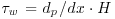 . Based on this velocity (
 ) and the flow depth (H), this corresponded to a friction Reynolds number of Reτ ≈ 1,200. Figure 12.3 presents the set-up of the permeable-bed simulation (PBS). The permeable bed consisted of three layers of spheres arranged in a cubic packing, placed on a smooth wall.
Figure 12.3 Computational domain and arrangement of porous bed comprised of spheres for the LES of flow over a permeable bed.
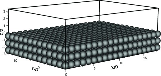
The computational domain of the PBS spanned over 5.3H × 3.5H × (H + 3D) and included the surface flow region (H) and the subsurface region consisting of the three layers of spheres (Figure 12.3). The computational domain of the impermeable bed simulation (IBS) spanned 6.12H × 3.06H × (H + 0.5D). The size of the domain was chosen to be large enough to include all relevant turbulence structures, and was close to the often-adopted 2πH × πH × H domain size for smooth-bed flows. High-resolution grids were employed consisting of 75 (PBS) and 91 (IBS) million grid points in total. The grid was Cartesian and each sphere/hemisphere was resolved explicitly using 40 grid points over the diameter in the horizontal and 60/30 grid points in the vertical direction. Based on the friction velocity, the grid spacings in terms of wall units were Δx+ ≈ 7 in the streamwise direction, Δy+ ≈ 7 in the spanwise direction and Δz+ ≈ 1.0-2.0 close to the top of the spheres/hemispheres. Both flows were considered fully developed and in an infinitely wide domain, which allowed application of periodic boundary conditions in the streamwise and spanwise directions. In both LES models, the free surface was set as a frictionless rigid lid and treated as a plane of symmetry, a reasonable approximation considering the low Froude number (Fr ≈ 0.17) of the flows and hence the absence of any significant surface waves. On both the sphere/hemisphere surfaces and the wall between the hemispheres, the no-slip condition was applied, and in the case of the spheres/hemispheres this was accomplished by employing the third-order accurate immersed boundary method of Peller et al. (2006). Additional simulations were carried out for the flow over a smooth bed in order to directly compare the turbulence statistics between a rough bed flow and its smooth bed counterpart (see Figure 12.5). The smooth bed simulation (SBS) featured a domain size and grid spacings in the horizontal that were similar to the rough bed simulations, but were sufficiently fine near the smooth wall, with Δz+ ≈ 1, to justify the no-slip treatment of the smooth wall. In all simulations, the dynamic Smagorinsky model (Germano et al., 1991) was employed as the SGS model.
Figure 12.4 (a) Contours of instantaneous streamwise velocity fluctuation (u′) in a 2D plane approximately ten wall units above a smooth wall; (b) spanwise distribution of autocorrelations of the three velocity fluctuation components at approximately ten wall units above a smooth wall.
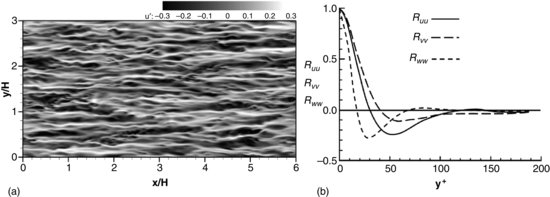
Figure 12.5 Flow over a hemispherical bed: (a) time- and spatially- averaged streamwise velocity profiles obtained from LES and data of previous experimental studies (Grass et al., 1991; Dancey et al., 2000) and DNS (Singh et al., 2007). Here, u+ = <u>/u* and  . (b) Calculated and measured profiles of the streamwise turbulence intensity. Symbols are from experiments except for Singh et al. (2007) which is from DNS. The hemisphere top is located at z/h = 0.028.

Figure 12.4a shows the instantaneous streamwise velocity fluctuations in a 2D plane approximately ten wall units above the smooth wall. The presence of streaks is clearly visible, and high (white) and low (black) velocities are ordered in an alternating fashion. The longest streaks are approximately half the size of the domain and they are regularly spaced in the spanwise direction. Generally, low- and high-speed streaks are a result of counter-rotating, near-wall, vortex pairs with size σ (as sketched in Figure 12.1b), which entrain high-momentum fluid into a high speed streak and low momentum fluid into a low speed streak. Figure 12.4b presents the spanwise distribution of two-point correlation of the streamwise, spanwise and wall normal velocity fluctuations, Ruu, Rvv, Rww, which allows quantification of the important length-scales of low- and high-speed streaks. The two-point correlation of the streamwise velocity fluctuation, Ruu, allows quantification of the streak spacing, λ, and the two-point correlation of the wall-normal velocity fluctuation, Rww, allows the determination of the average vortex roller size, σ, (Rajaee et al., 1995). Ruu gives the spanwise distance between a high-speed and a low-speed streak, i.e. λ/2 (Kim et al., 1987) and in Figure 12.4b Ruu reaches a minimum at a distance y+ = 50, suggesting an average streak spacing of λ+ = 100. The spanwise location of the minimum of Rww gives the average vortex roll size, which for this flow is found to be σ = 30 wall units.
The validation of the rough-bed simulations was accomplished by comparing time-averaged velocity, streamwise and vertical turbulence intensity and shear stress profiles with measurement data, for which very good agreement between LES and measurements was found. Figure 12.5a presents profiles of the time- and spatially averaged streamwise velocity from the smooth and rough bed LES study of Bommiyanuni and Stoesser (2011) together with experimental data on a Clauser plot. Also plotted in Figure 12.5a are the results of the LES of channel flow over a smooth bed, which illustrates the effect of roughness on the velocity distribution (i.e. a downshift of the profile). The roughness Reynolds number of the LES is estimated to be 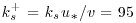 , where ks is the equivalent grain roughness. It can be seen that the LES results for ks+ = 95 agree quite well with the measured data for ks+ ≈ 100 and the results follow the log-law distribution for ks+ = 95 quite accurately. The vertical distribution of the spatially averaged (in horizontal planes) streamwise turbulent fluctuations (urms normalized by the global bed-shear velocity u*) are plotted in Figure 12.5b, together with data from the DNS of Singh et al. (2007) and various experiments. It can be observed that the overall agreement between the LES results and the experimental/numerical data is fairly good. Comparison of the rough and smooth channel results indicates that the bed roughness influences the streamwise turbulence intensity over the entire channel depth. At regions close to the bed, the streamwise turbulence intensity is higher in the smooth channel but falls below the rough wall as the distance from the bed increases. The peak in the spatially averaged turbulence intensity profile is located almost exactly at the tops of the roughness.
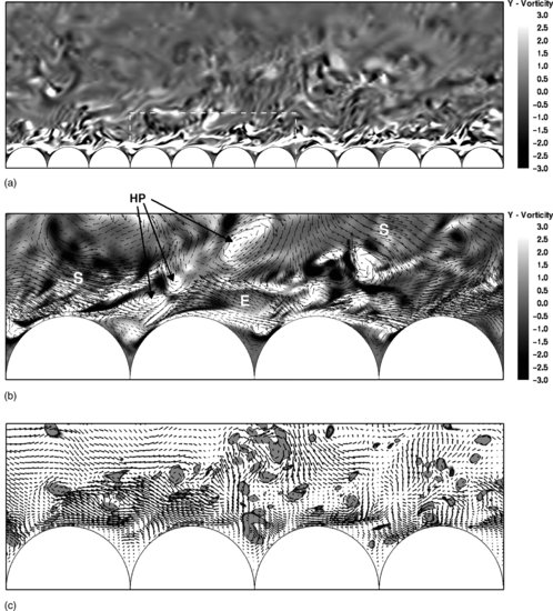
Bommiyanuni and Stoesser (2011) educed the structure of turbulence over a rough, impermeable bed using contours of spanwise vorticity, velocity perturbation vectors and contours of the swirl strength in a longitudinal plane through the centre of the hemispheres. Areas of nonzero vorticity throughout the flow depth (Figure 12.6a) qualitatively show the presence of vortex structures in the flow. In regions close to the bed, the majority of positive values of the contour levels indicate vertical shear (du/dz), but may also suggest that these vortex structures are rotating preferentially in a clockwise direction. Although turbulence intensities decrease with increasing distance from the bed, vortical motion is still visible close to the water surface. Figure 12.6b shows a detailed view of the flow near the rough bed and, in addition to vorticity contours, the velocity perturbation vectors are also plotted. Besides the vortical motion, sweep (i.e. u′ > 0 and w′ < 0) and ejection (i.e. u′ < 0 and w′ > 0) events, the dominant structures of turbulence that are mainly responsible for turbulent momentum transfer near the bed can be identified. For instance, in Figure 12.6b such momentary events are marked with E (for ejection) and S (for sweep), during which near-bed fluid is ejected into the boundary layer flow and high momentum outer layer fluid is swept towards the roughness elements. Sweeps and ejections are accompanied by hairpin vortices, which are labelled as HP in Figure 12.6b. A more quantitative way of identifying the signatures of hairpin vortices is to plot the swirl strength, which is computed using a reduced tensor that contains only the in-plane velocity gradients (Adrian et al., 2000). Contours of the two-dimensional swirl strength isolate regions that are swirling about the axis normal to the plane. Figure 12.6c presents contours of the swirl strength, together with perturbation vectors, at an instant in time and reveals that a number of vortices, possibly hairpin packets, can be identified and their distribution is similar to that observed by Adrian (2007).
Figure 12.6 (a) Contours of instantaneous spanwise vorticity in the flow over hemispheres; (b) blow-up of a region in which the vorticity contours are overlaid by vectors of the velocity fluctuation; (c) contours of the swirl strength and velocity fluctuations at the same instant in time.
The existence of hairpin vortices, and others, is supported by the three-dimensional visualization of these vortical structures, through an iso-surface of a Galilean-invariant Q (Hunt et al., 1988), which is defined as:
(12.4) 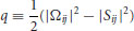
where 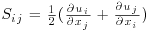 is the rate of the strain tensor and
  is the vorticity tensor. Hunt et al. (1988) defined a vortex as a region with Q > 0, in which the pressure attains a local minimum and hence as a local region in which vorticity dominates shear strain, allowing rotation and shear be to distinguished.
In the preliminary studies of Bommiyanuni (2010), the dominant coherent structures of flow over a single hemisphere were educed using the Q-criterion (Figure 12.7). The oncoming laminar boundary layer flow was free of large-scale flow structures and thus provided a clear look at the structures that evolve as a result of the obstacle. Figure 12.7 reveals a number of structures. Upstream of the hemisphere, a horseshoe vortex (HSV) forms as the boundary layer flow separates in front of the hemisphere, leading to a multi-component horseshoe vortex system that features several secondary vortices (sHSV). Behind the hemisphere, hairpin vortices (HP-1, HP-2 and HP-3) evolve as a result of shear between the outer flow and the recirculation zone. The hairpin vortices grow as they travel downstream. The legs of the horseshoe vortex contain significant streamwise vorticity, very similar to the vortex tubes in high- and low-speed streaks, which also results in the generation of hairpin vortices. These secondary hairpin vortices (sHP) are considerably smaller than those evolving in the lee of the hemisphere.
Figure 12.7 Turbulent flow structures over a hemisphere visualized by the Q-criterion.
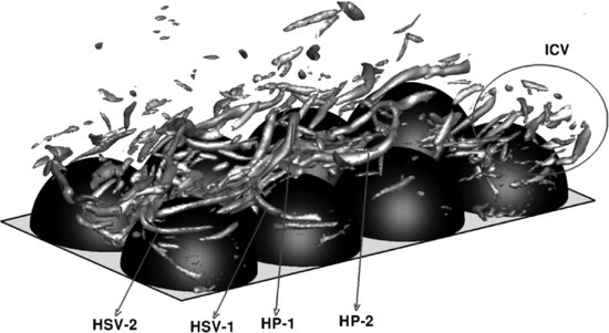
Figure 12.8 presents a snapshot of the iso-surface of Q over a selected region of the hemispherical bed in which structures can be identified very similar to those discussed in conjunction with Figure 12.7, such as the hairpin structures marked as HP-1 and HP-2. A number of elongated structures also exist, which are either remaining legs of hairpin vortices or streamwise vortices from which secondary hairpin vortices evolve. Between the hemispheres, several spanwise vortices can be seen, possibly being generated from flow separation at the crests of upstream hemispheres. Also present are horseshoe vortex type structures (indicated as HSV-1 and HSV-2 in Figure 12.8) that are generated in a manner similar to the horseshoe vortex system in Figure 12.7; here the vertical location of these HSVs coincides with the virtual bed position. Animations of the flow (see Animations S1, S2 and S3 on the Wiley web site, www.wiley.com/go/venditti/coherentflowstructures) reveal that there is quite a strong interaction between the above mentioned structures, as well as with sweep and ejection events. For instance, a hairpin vortex is formed at one crest of a hemisphere but is then broken up into smaller incoherent vortices (ICV), most likely by a sweep event.
Figure 12.8 Turbulent flow structures over a rough bed comprised of hemispheres visualized by the Q-criterion.
The turbulent flow structures identified over the permeable bed (Figure 12.9) are similar to those discussed above, although here the flow is additionally influenced by significant mass exchange between the fast-moving outer flow and the slow-moving subsurface flow. Figure 12.9 presents a snapshot of the complex velocity perturbation field, providing insight into the prevailing turbulent flow structures. At the time instant shown, there are strong ejections away from the interface, while at other instances sweeps towards the interface are observed. These events are the main driver for hyporheic exchange, as they force fluid out of the cavities between spheres (during ejection) and promote inrushes of ‘fresh’ fluid into the bed during sweeps.
Figure 12.9 Perturbation vectors (u′–w′) in selected longitudinal planes with (a) minimum and (b) maximum porosity.

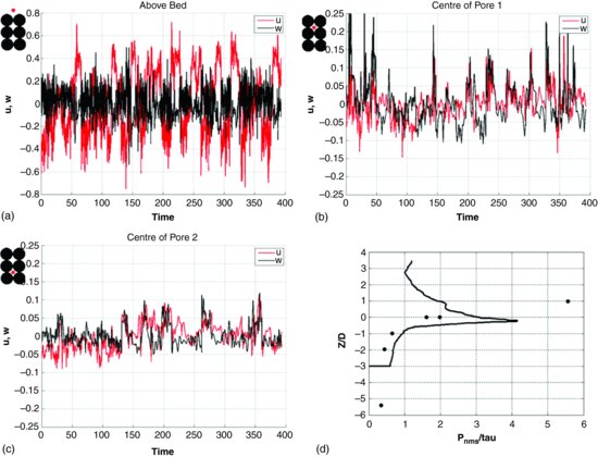
The raw velocity time signals plotted in Figure 12.10 provide evidence of the highly fluctuating nature of the flow not only above the permeable bed (Figure 12.10a), but also within the pores, and in particular in the first pore below the bed surface (Figure 12.10b). Even in the second pore (Figure 12.10c), turbulence is still visible but is already damped considerably compared to the flow above the bed. The recurrence of strong sweeps and ejections is particularly obvious from the velocity signal outside the bed (Figure 12.10a), and sweeps and ejections are still visible in the first pore (Figure 12.10b). The damping of turbulence is quantified by the distribution of pressure fluctuations depicted in Figure 12.10d. This curve has a pronounced peak slightly below the top of the spheres, which is where the maximum pressure forces on the spheres are found. For comparison, the experimental data of Detert et al. (2010) are also included in the plot, which were obtained by measuring pressure signals in a naturally packed gravel bed. The simulated and measured decay of pressure fluctuations with depth in the bed are very similar and follow an exponential curve. However, the level of pressure fluctuations in the experiment is somewhat lower due to the much denser packing of natural gravel in comparison to the artificial sphere arrangement used in the LES. The large experimental value at z = D can be explained by the fact that this is a data point at a single location (probably exactly above a gravel clast), while the LES curve represents a spatial average. However, values of pressure fluctuations up to six times larger than the mean wall shear stress were also observed at individual locations in the LES. An animation of this flow field (Animation S4 on the Wiley web site) provides a very good visualization of such flows.
Figure 12.10 Raw time signals of the streamwise (black line) and wall normal (red line) velocity fluctuation (a) above the porous bed; (b) in the centre of pore 1; (c) in the centre of pore 2; (d) spatially-averaged vertical distribution of pressure fluctuations. Continuous line: LES; symbols: experiment of Detert et al. (2010).
12.3.2 Flow through vegetation
The flow through partially vegetated channels, or emergent and submerged vegetation, is characterized by significant velocity gradients (laterally, longitudinally and vertically) that result in shear layer formation and generation of large-scale turbulent flow structures. A large number of experimental studies have aimed to quantify flow resistance in terms of a drag force (e.g. Stone and Shen, 2002; Tanino and Nepf, 2008), with some experimental works examining the flow field and turbulence structure within a plant canopy (Nepf and Vivoni, 2000; Lopez and Garcia, 2001; Ghisalberti and Nepf, 2002; White and Nepf, 2008; Liu et al., 2008). To date, very little numerical work has been reported of these flows and most of these studies have been based on the Reynolds-averaged-Navier–Stokes (RANS) equations (Naot et al., 1996; Fischer-Antze et al., 2001; Choi and Kang, 2001; Neary, 2003). Although the time-averaged flow was predicted well using RANS models, they were less successful at predicting turbulence-related quantities, due to the fact that RANS models cannot accurately account for the organized large-scale unsteadiness and asymmetries (coherent structures) induced by the local flow-vegetation interactions. Cui & Neary (2008) and Stoesser et al. (2009, 2010) have demonstrated that large-eddy simulation (LES) can be employed to elucidate the large-scale coherent structures present in flow through idealized vegetation and showed the excellent predictive capabilities of LES for the turbulence statistics of such flows. An example of the utilization of LES to predict flow through idealized emergent vegetation is presented herein. Stoesser et al. (2010) resolved the flow around individual cylinders comprising a vegetated area by using a high-resolution grid through which each vegetation element was explicitly represented, so that pressure and the frictional drag could be computed directly.
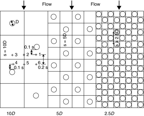
In the LES of Stoesser et al. (2010) simulated time-averaged velocity and turbulence intensity profiles were first compared with laboratory data to validate the approach and chosen grid resolution. Then the LES was used to investigate the effects of vegetation density and cylinder Reynolds number on flow resistance, as well as on the time-averaged and instantaneous flow fields. The simulation setup of the validation case was chosen to match the experiments conducted by Liu et al. (2008), who placed a matrix of rigid cylinders in a staggered arrangement into a rectangular flume and conducted detailed LDA measurements at six verticals within the flow (Figure 12.11, where s is defined as the distance between two cylinders in the streamwise direction, with s = 10D in the experiment of Liu et al. (2008)). The vegetation density, φ, herein defined as the volume that is occupied by the cylinders over the total volume, was φ = 0.0157. The cylinder Reynolds number based on the bulk velocity, ubulk, and the cylinder (stem) diameter, D, was ReD = 1340. In addition to the 10D case of Liu et al. (2008), LES were carried out at two additional vegetation densities of s = 5D and s = 2.5D, or φ = 0.0628 and φ = 0.2513, respectively (Figure 12.11) and at one additional (lower) stem Reynolds number of ReD = 500. In total, six different numerical experiments were performed. The computational flow domain chosen was the same for all cases and spanned 20D, 10D and 10.22D (corresponding to the water depth) in the streamwise, spanwise and vertical directions respectively. The details of each grid for the six numerical experiments are omitted for brevity herein and can be found in Stoesser et al. (2010). The no-slip condition at the bed and at the cylinder surfaces was applied, which was justified by the fact that the first grid point above the wall was situated well within the viscous sublayer. Periodic boundary conditions were applied in the streamwise and spanwise directions, and the free surface was set as a frictionless rigid lid at which a zero-stress boundary condition was used.
Figure 12.11 Flow domain and cylinder arrangement for the three different setups of flow through emergent vegetation. The six measurement locations of the experiment are also depicted.
In the validation phase of the study, Stoesser et al. (2010) compared LES-calculated time-averaged streamwise and vertical velocities, and streamwise turbulence intensity profiles, with those measured in the experiments of Liu et al. (2008) at six locations. Figure 12.12a shows these comparisons for the streamwise velocity (solid lines represents the LES for the 10D case and the dots the experimental data) at three selected locations. The agreement of the LES with the experiment is very good, and it is noteworthy that the LES is able to reproduce accurately the near-bed bulge (indicated by the arrow in Figure 12.12) in the streamwise velocity profile. This bulge results from the prevailing secondary flow that entrains high momentum fluid into the wake behind the cylinders near the bed. Figure 12.12b presents profiles of the streamwise turbulence intensity at the same locations, and again agreement between LES and experimental data is very good. It is remarkable that the streamwise turbulence intensity increases considerably as a result of denser vegetation, particularly along vertical 5, which is a result of streamwise velocity gradients that are present in dense vegetation and almost absent in flows through low-density vegetation.
Figure 12.12 Simulated and measured profiles of: (a) streamwise velocity, and (b) streamwise turbulence intensity at selected locations.
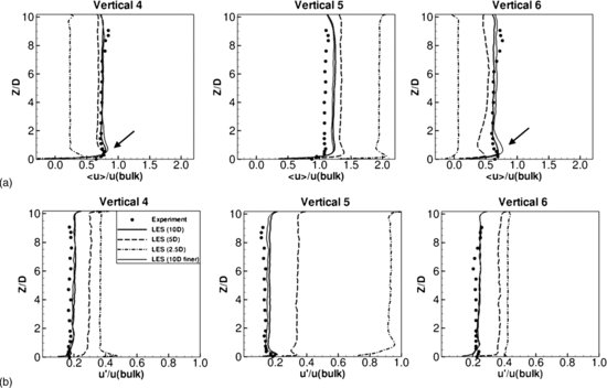
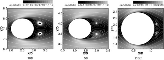
Figure 12.13 presents contours of the time-averaged streamwise velocity and streamlines at about half depth for the three different densities investigated. While in the 10D and 5D cases a clear wake behind the cylinder and an area of higher velocities between the cylinders can be identified, the 2.5D flow field exhibits large velocity gradients in both the streamwise and spanwise directions. The streamlines reveal that the 10D and 5D cases exhibit similar flow features, including flow separation at approximately 90° and a relatively large recirculation region that consists of two counter-rotating vortices that have about the length of the cylinder diameter. However, in the 2.5D case, the flow separates considerably later (at approximately 130°) and the recirculation region behind the cylinder is much smaller than the ones found behind the cylinders spaced at 10D and 5D. The length of the vortex pair behind the 2.5D case cylinder is approximately only 0.25 of the cylinder diameter.
Figure 12.13 Contours of time-averaged streamwise velocity in a horizontal plane at z/D = 0.5 together with streamlines around the cylinder for the three cases at ReD = 1340.
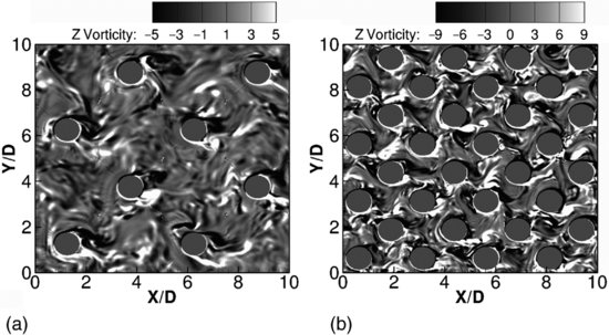
The benefits of employing LES for such flows are not only that it reproduces reliably and accurately the turbulence statistics and acting forces of complex 3D flows, but also that LES allows study of the instantaneous flow and thereby reveals important physical mechanisms and relationships. The horizontal distribution of vertical vorticity (z-vorticity) at an instant in time and in a plane at approximately half the water depth (z = 5D) for two vegetation densities is presented in Figure 12.14. The flow through less dense vegetation (here the s = 5D case is depicted in Figure 12.14(a) is characterized by regular vortex shedding. High levels of vertical vorticity are found close to the cylinder, but these decrease as the vortices are convected downstream. As the density of vegetation increases, the vortex shedding at the cylinders is influenced by upstream vortices, thereby resulting in a more irregular shedding behaviour. This is supported by elevated levels of vertical vorticity, which is now also found on the upstream side of the cylinders in the 2.5D case (Figure 14.14b). Animations of the flow field for the 5, 10 and 2.5D cases (Animations S5, S6, S7 on the Wiley web site) well illustrate the dynamics of flow in these differing cylinder densities.
Figure 12.14 Snapshot of vertical vorticity contours in a horizontal plane at half channel depth for two vegetation densities: (a) 5D and (b) 2.5D. (Note that the 2.5D case has a different vorticity scale.)
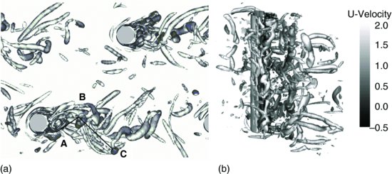
An impression of the large-scale 3D vortical structures behind the cylinders can be obtained from instantaneous iso-surfaces of the pressure perturbation p′ = (p − <p>)/(ρU∞). Snapshots showing such iso-surfaces in an oblique view for the 10D and 2.5D cases are presented in Figure 12.15. For the 10D case (Figure 12.15(a)), vertical vortices are observed on the sides of the cylinder originating from the separated shear layer behind the cylinder. The vortices extend over the full cylinder height and exhibit similar features to von Kármán vortices behind long isolated cylinders, where the shear layers roll up and trigger regular alternating shedding of vortices. In the 2.5D case (Figure 12.15b), the process is influenced strongly by the flow acceleration between cylinders and the presence of vortices that are shed at upstream cylinders, which alters the shedding process and structure of the vortices. As a result, the vortices do not extend over the entire water depth and appear to be incoherent. Snapshots of three-dimensional turbulent flow structures visualized with iso-surfaces of the Q-criterion (Hunt et al., 1988) for the 10D case from above (Figure 12.16(a)) and from an oblique view (Figure 12.16(b)) illustrate that the regular shedding of von Kármán vortices is clearly visible (indicated by lines connecting A-B-C, Figure 12.16a). While these structures exhibit some two-dimensionality in their early stage, they are stretched in the streamwise direction while being convected downstream. Packets of smaller vortices evolve, although these vortices lose their coherence and weaken before reaching the downstream cylinder (Figure 12.16(b)).
Figure 12.15 Isosurfaces of pressure fluctuations for two vegetation densities (a) 10D and (b) 2.5D.
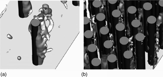
Figure 12.16 Instantaneous isosurfaces (shaded by the streamwise velocity) of the Q-criterion for the three vegetation densities for the 10D case: (a) Top view; (b) Oblique view.
12.3.3 Flow over dunes
The flow over dunes in sand-bed rivers has been studied widely in order to understand the hydrodynamics and turbulence, and the mechanisms of bedload and suspended-load transport. The importance of the hydrodynamic and geomorphological impact of bedforms in rivers is reflected in numerous experimental studies on dunes undertaken by Müller and Gyr (1986), Bennett and Best (1995), Mierlo and de Ruiter (1988), Lyn (1993), Coleman and Melville (1996), Kadota and Nezu (2002), Hyun et al. (2003), Maddux et al. (2003a,b) as well as many others. A wide range of configurations have been investigated and progress has been made in understanding the mean flow and turbulence as well as the sediment transport characteristics (an extensive summary is given in a detailed review by Best, 2005). The presence of dunes at the bed causes the flow to separate at the dune crest and a separation zone is created in the leeside of the dune (Figure 12.1c). Associated with flow separation is a shear layer from which a number of coherent structures evolve. The geomorphological origin of ripples and dunes is believed to lie in the presence of these coherent structures, which are the driving mechanism for sediment transport and hence for bed deformation processes. Coherent flow structures are difficult to detect experimentally as they vary strongly in space and time. Ideally, experimental investigations should be complemented with numerical simulations for further exploration of the mechanisms of instantaneous flow over bedforms, but also to serve as predictive tools to perform parametric studies. Until very recently, only a few numerical simulations of flow over dunes existed, which were mainly based on RANS methods (e.g. Mendoza and Shen, 1990; Yoon and Patel, 1996). Such RANS models can capture much of the mean-velocity information but cannot reproduce large-scale flow structures. Recent work has applied LES to flow over dunes (Yue et al. 2005, 2006; Stoesser et al., 2008; Grigoriadis et al., 2009; Omidyeganeh and Piomelli, 2011), in which turbulence statistics were predicted accurately and all relevant turbulence structures over dunes, including rollers, kolk-boil vortices, splats and streaks, were revealed.
Some results of the LES of flow over two-dimensional dunes by Stoesser et al. (2008) and Omidyeganeh and Piomelli (2011) are presented here. The set-up of the two LES was selected to complement the laboratory experiments undertaken by Polatel (2006). In these experiments, a train of 22 two-dimensional, fixed, dunes was attached to the bottom of a flume. The dune height was k = 20 mm, and the dune wavelength was λ = 400 mm, so that λ/k = 20, which is in accordance with many previous studies and with dune shapes found in rivers. The LES study featured a dune-length: water-depth ratio of λ/h = 5 (or water-depth: dune-height ratio of h/k = 4) and the Reynolds number Re, based on the average bulk velocity ubulk ≈ 0.3 m s−1 and the maximum flow depth h, was approximately Re = 25,000. Velocity measurement data were available and were used for comparing numerical simulation and experiments. The computational domain of Stoesser et al. (2008) spanned one dune length λ in the streamwise, 4h in the spanwise and h in the vertical direction, respectively. The domain of Omidyeganeh and Piomelli (2011) also spanned one dune length, but their spanwise dimension was twice that of Stoesser et al. (2008). The grid of Stoesser et al. (2008) consisted of 416 × 170 × 128 grid points in the streamwise, spanwise and vertical directions, respectively, with a maximum grid spacing in terms of wall units of Δx+ ≈ 20 in the streamwise direction, Δy+ ≈ 19 in the spanwise direction and Δz+ ≈ 1 near the dune surface. Omidyeganeh and Piomelli (2011) used the same number of grid points in streamwise and wall normal directions and employed approximately two times the number grid points in the spanwise direction to Stoesser et al. (2008) because of their wider domain. Both LES resolved the near-wall flow with 3-6 points in the viscous sublayer, which justified the use of a no-slip wall condition. Additionally, in both LES, the free surface was treated as a flat plane of symmetry (with zero stress condition) and periodic boundary conditions were applied in the streamwise and spanwise directions. Both LES used the dynamic model to compute SGS stresses, and whilst Stoesser et al. (2008) used local averaging to obtain the Smagorinsky coefficient, Omidyeganeh and Piomelli (2011) made use of the Lagrangian averaging technique proposed by Meneveau et al. (1996).
Figure 12.17(a) presents streamlines visualizing the time-averaged flow and the size of the mean recirculation zone that forms behind the dune crest. Figure 12.17(b) compares measured and simulated time-averaged streamwise velocities along the six measurement verticals, which are drawn into Figure 12.17(a). The data of Omidyeganeh and Piomelli (2011) are represented by the solid line, while that of Stoesser et al. (2008) is represented by the dashed line. The overall agreement is good for both simulations and the two LES are virtually identical. In Figure 12.17(c), the Reynolds shear stress is compared along the six verticals and again an overall very good agreement was obtained with the experimental data.
Figure 12.17 (a) Streamlines of flow and location of six measurement verticals at which statistical quantities are compared; (b) measured (dots) and simulated time-averaged streamwise velocities; (c) measured and simulated Reynolds-shear-stresses along the six measurement verticals. The solid line represents the LES data of Omidyeganeh and Piomelli (2011), the dashed line represents the LES data of Stoesser et al. (2008). Reprinted from Omidyeganeh, M. and Piomelli, U. 2011, with permission from Taylor & Francis Group.
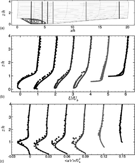
Figure 12.18 displays the turbulent flow structures from the simulations of Stoesser et al., (2008, Figure 12.18a) and Omidyeganeh and Piomelli (2011, Figures 12.18b and 12.18c) at selected instants in time, as visualized by isosurfaces of the instantaneous pressure fluctuation. Spanwise vortices (rollers) are generated in the shear layer separating from the crest due to a Kelvin–Helmholtz (K–H) instability. These vortices are convected downstream and either interact with the wall and then rise to the surface, as a so-called kolk-boil vortex (denoted HP in Figure 12.18a and circled in Figures 12.18b and (c), or are convected along the separating shear layer while diffusing. The kolk boil vortices usually take the form of a horseshoe or a hairpin, and Figures 12.18b and 12.18c visualize the horseshoe-shaped kolk-boil vortex as it rises to the surface. Eventually, the vortex reaches the water surface (Figure 12.18c) and creates an upwelling there, as a so-called boil. The vortex is originally vertical, but is later tilted at an angle of 40-60 degrees with respect to the vertical axis. Similar visualizations of, and findings on, the kolk-boil vortex system were reported in Grigoriadis et al. (2009), who performed a large-eddy simulation of flow over a similar 2D dune to that reported herein. An animation of an isosurface of a pressure-fluctuation that visualizes the generation and fate of spanwise rollers, as well as the generation and fate of a kolk-boil vortex, can be accessed at Animation S8 on the Wiley web site.
Figure 12.18 Flow over dune bedforms: turbulence structures at selected instants in time visualised with isosurfaces of pressure fluctuation. (b and c reprinted from Omidyeganeh, M. and Piomelli, U. 2011, with permission from Taylor & Francis Group.

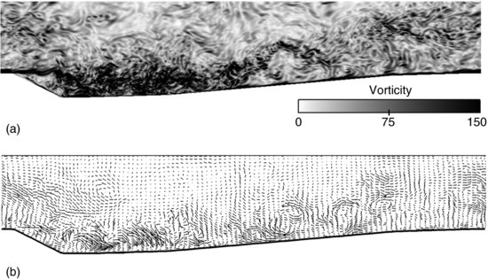
Figure 12.19 presents snapshots of the flow visualized by contours of the vorticity magnitude (Figure 12.19a) and instantaneous velocity perturbation vectors (Figure 12.19b) in a longitudinal plane at an instant in time. An animation of Figure 12.19a can be found at Animation S9 on the Wiley web site. The vortex rollers are visualized springing off the crest of the dune and an area of high vorticity is visible downstream of the crest. Turbulence is strongest in the reattachment region, which is where most rollers impinge on the bed, generating kolk-boil vortices. These latter vortices are then convected towards the water surface where they eventually impinge as a boil.
Figure 12.19 (a) Distribution of the magnitude of the vorticity vector at an instant in time; (b) instantaneous velocity perturbation vectors in a selected longitudinal plane.
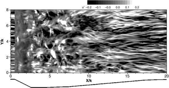
Instantaneous velocity vectors in a wall-parallel plane at approximately Δz+ ≈ 10 are presented in Figure 12.20(a). Most turbulence occurs in the vicinity of the time-averaged location of reattachment (x/k ≈ 5). The points of instantaneous reattachment are identified by areas of strongly diverging vectors (i.e. singular points) and of high pressure (Figures 12.20(b) and 12.20(c)), where impinging fluid is reoriented in all directions tangential to the wall. These ‘splats’ are a result of the impermeability condition of the wall, with the consequence of the wall-normal component of turbulent kinetic energy being transferred to the tangential components. In this region, the spanwise fluctuations were found to be of the order of the streamwise fluctuations or even higher (Stoesser et al., 2008). Further downstream of the mean reattachment region, the footprints of vortices that are convected downstream are revealed by smaller splats as well as areas of streaks, so that areas of high and low instantaneous pressure exist (Figure 12.20(c)). Further downstream, these vortices are lifted upwards as the boundary layer grows and the splats disappear, while the near-wall streaks remain and become similar, in terms of size and spacing, to the streaks observed above smooth walls (Figure 12.4a). This can also be seen clearly in Figure 12.21, where instantaneous streamwise velocity fluctuations in a wall-parallel plane near the bed are visualized. Again, in the region of mean reattachment, strong velocity fluctuations without a clear structure are observed, and further downstream from about x/k ≈ 10 elongated streamwise structures appear, which represent high and low speed streaks that begin to form and are established as the boundary layer grows towards the next crest. The animation of this near-wall flow (Animation S10 on the Wiley web site) best illustrates this behaviour and provides a vivid impression of the reattachment and the re-organization of the flow, as well as the formation of high- and low-speed streaks, as the new boundary layer is established towards the next dune crest.
Figure 12.20 (a) Distribution of instantaneous velocity vectors in a wall-parallel plane near the bed; (b) and (c) blow-ups at selected locations showing velocity vectors and contours of high (dark areas) and low (light areas) pressure.
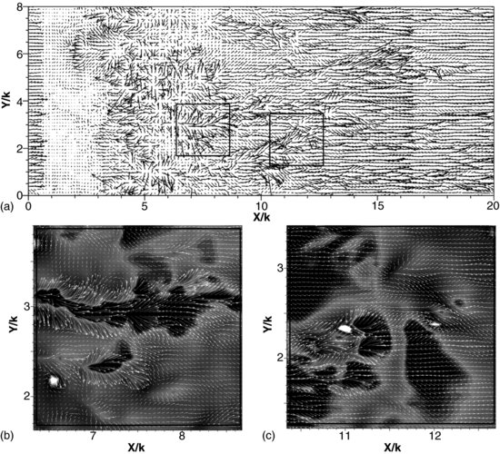
Figure 12.21 Distribution of instantaneous streamwise velocity fluctuations in a wall-parallel plane near the bed at Δz+≈ 10.
12.4 Conclusions
In this chapter, the method of large-eddy simulation has been introduced, and it was shown that LES can be applied successfully to open-channel geophysical flows, revealing coherent flow structures, their generation and fate, and allowing quantification of their contribution to the turbulence statistics. In the three examples presented here, it was shown that LES not only yields information on the complex time-averaged flow, but also educes the unsteady features by resolving the large-scale eddies of turbulence, thereby providing insights into the physics of such flows.
Flow over smooth beds is characterized by near wall-streaks and streamwise vortices from which hairpin vortices erupt into the outer layer, triggering sweeps and ejections. The rough and permeable bed flows exhibit similar features, but local flow separation and recirculation zones behind penetrating roughness elements create a number of additional coherent flow structures, including horseshoe vortices, primary and secondary hairpin vortices and, in case of the permeable bed, in- and out- flux events into and out of the subsurface pores. These additional flow structures are disruptive to streaks and hence flow over rough and permeable beds is less organized than that over smooth beds. Flow through emergent vegetation is characterized by vortex shedding behind individual stems and vegetation density is found to be a key parameter determining the type of coherent flow structures that occur. Whilst vortex shedding occurs regularly at low to moderate vegetation densities, similar to flow around an isolated obstacle, shedding becomes irregular at high vegetation densities due to the interaction with vortices shed from upstream stems and the presence of strong streamwise and spanwise velocity gradients. The flow over two-dimensional dunes is characterized by a distinct spanwise vortex, or roller, which originates at the dune crest as a result of flow separation and shear layer formation. The roller reattaches in the lee of the dune, where it triggers a kolk-boil vortex of the shape of a horseshoe or hairpin, which rises to the water surface, where it eventually creates a boil. The flow organizes itself on the growing boundary layer on the stoss side of the next dune, while forming low- and high- speed streaks in a similar manner to flow over smooth beds.
The details that can be obtained from a LES are important for furthering our understanding of the physical mechanisms, such as those responsible for local scouring, erosion and deposition, and ultimately evolution of the fluvial landscape. The time-dependent LES are computationally expensive, but they are affordable on modern high-performance computers and increasingly on PC clusters. However, as of today, well-resolved LES are feasible only for problems with relatively low Reynolds numbers or at smaller scales, such as laboratory-scale flows. At high Reynolds numbers, as usually found in most geophysical flows and engineering practice, the near-wall region cannot be resolved at a reasonable cost. Low-cost alternatives to LES, such as detached-eddy simulation (DES) or partially averaged Navier Stokes (PANS) techniques are being developed, validated and tested. On the other hand, such approaches involve more than just subgrid-scale modelling and hence will lead to uncertainties, requiring thorough validation on a case-to-case basis. As a final point, there is a clear trend that, because available computer power will continue to increase, LES will, in the not-too-distant future, be used for large-scale, open-channel flow calculations.
References
Adrian, R.J. (2007) Hairpin vortex organization in wall turbulence. Physics of Fluids 19, 041301. DOI: 10.1063/1.2717527.
Adrian, R.J., Christensen, K.T. and Liu, Z.C. (2000) Analysis and interpretation of instantaneous turbulent velocity fields. Experiments in Fluids 29, 275–290.
Bennett, S.J. and Best, J.L. (1995) Mean flow and turbulence structure over fixed, two-dimensional dunes: implications for sediment transport and bedform stability. Sedimentology 42, 491–513.
Best, J.L. (2005) The fluid dynamics of river dunes: a review and some future research directions. Journal of Geophysical Research 110, F04S02. DOI: 10.1029/2004JF000218.
Bezzola, G.R. (2002) Fliesswiderstand und Sohlenstabilität natürlicher Gerinne unter besonderer Berücksichtigung des Einflusses der relativen Überdeckung. Ph.D. thesis, Eidgenossische Technische Hochschule, Zurich.
Bommiyanuni, S. (2010) Large Eddy Simulation of Turbulent Flow over a Rough Bed using the Immersed Boundary Method. M.S. thesis, Georgia Institute of Technology, Atlanta, GA.
Bomminayuni S. and Stoesser T. (2011) Turbulence statistics of open-channel flow over a rough bed. Journal of Hydraulic Engineering 137, 1347–1358.
Choi, S.U. and Kang, H. (2004) Reynolds stress modeling of vegetated open channel flows. Journal of Hydraulic Research 42, 3–11.
Coleman, S. and Melville, B. (1996) Initiation of bed forms on a flat sand bed. Journal of Hydraulic Engineering 122, 301–310.
Corino, E.R. and Brodkey, R.S. (1969) A visual investigation of wall region in turbulent flow. Journal of Fluid Mechanics 37, 1–30.
Cui, J. and Neary V.S. (2008) LES study of turbulent flows with submerged vegetation. Journal of Hydraulic Research 46, 307–316.
del Álamo, J.C. and Jiménez, J. (2003) Spectra of very large anisotropic scales in turbulent channels. Physics of Fluids 15 (6), L41–L44.
Dancey, C.L., Balakrishnan, M., Diplas, P. and Papanicolaou, A.N. (2000) The spatial inhomogeneity of turbulence above a fully rough, packed bed in open channel flow. Experiments in Fluids, 29, 402–410.
Detert, M., Nikora, V. and Jirka, G.H. (2010) Synoptic velocity and pressure fields at the water-sediment interface of streambeds. Journal of Fluid Mechanics 660; 55–86.
Ferziger, J.H. (1996) Large eddy simulation. In Simulation and Modeling of Turbulent Flows (eds T.B. Gatski, M.Y. Hussaini and J.L. Lumley). Oxford University Press, Oxford, pp. 109–154.
Fischer-Antze, T., Stoesser, T., Bates, P.B. and Olsen, N.R.B. (2001) 3D numerical modelling of open-channel flow with submerged vegetation. Journal of Hydraulic Research 39, 303–310.
Germano, M., Piomelli, U., Moin, P. and Cabot, W. (1991) A dynamic subgrid-scale eddy viscosity model. Physics of Fluids A. Fluid Dynamics 3, 1760.
Ghisalberti M. and Nepf H.M. (2002) Mixing layers and coherent structures in vegetated aquatic flows. Journal of Geophysical Research 107, 3011. DOI: 10.1029/2001JC000871.
Grass, A.J. (1971) Structural features of turbulent flow over smooth and rough boundaries. Journal of Fluid Mechanics 50, 233–255.
Grass, A.J., Stuart, R.J. and Mansour-Tehrani, M. (1991) Vortical structures and coherent motion in turbulent flow over smooth and rough boundaries. Philosophical Transactions of the Royal Society A336, 33–65.
Grigoriadis, D.G.E., Balaras, E. and Dimas, A.A. (2009) Large-eddy simulations of unidirectional water flow over dunes. Journal of Geophysical Research 114, F02022. DOI: 10.1029/2008JF001014.
Hunt, J.C.R., Wray, A.A. and Moin, P. (1988) Eddies, Stream, and Convergence Zones in Turbulent Flows. Center for Turbulence Research, Stanford University, Report no. CTR-S88.
Hyun, B.S., Balachandar, R., Yu, K. and Patel, V.C. (2003) Assessment of PIV to measure mean velocity and turbulence in water flow. Experiments in Fluids 35, 262–267.
Jiménez, J., del Álamo, J.C., and Flores, O. (2004) The large-scale dynamics of near-wall turbulence, Journal of Fluid Mechanics 505, 179.
Kadota, A. and Nakagawa, H. (1997) Turbulent structure in unsteady depth-varying open-channel flows. Journal of Hydraulic Engineering 123, 752–763.
Kadota, A. and Nezu, I. (2002) Three dimensional structure of space-time correlation on coherent vortices generated behind dune crest. Journal of Hydraulic Research 37, 59–80.
Keylock, C.J., Hardy, R.J., Parsons, D.R. et al. (2005) The theoretical foundations and potential for large-eddy simulation (LES) in fluvial geomorphic and sedimentological research. Earth-Science Reviews 71, 271–304.
Kim, J. (1989) On the structure of pressure fluctuations in simulated turbulent channel flow. Journal of Fluid Mechanics 239, 157–194.
Kim, J., Moin, P. and Moser, R. (1987) Turbulence statistics in fully-developed channel flow at low Reynolds number. Journal of Fluid Mechanics 177, 133–166.
Kline, S.J., Reynolds, W.C., Schraub, F.A. and Runstadl, P.W. (1967) Structure of turbulent boundary layers. Journal of Fluid Mechanics 30, 741–773.
Lesieur, M. and Metais, O. (1996) New trends in large-eddy simulations of turbulence. Annual Review of Fluid Mechanics 28, 45–82.
Liu, D., Diplas, P., Fairbanks, J.D. and Hodges, C.C. (2008) An experimental study of flow through rigid vegetation. Journal of Geophysical Research 113, F04015. DOI: 10.1029/2001JC000871.
Lopez, F. and Garcia, M.H. (2001) Mean flow and turbulence structure of open channel flow through nonemergent vegetation. Journal of Hydraulic Engineering 127, 392–402.
Lyn, D.A. (1993) Turbulence measurements in open-channel flows over artificial bed forms. Journal of Hydraulic Engineering 119, 306–326.
Maddux, T.B., Nelson, J.M. and McLean, S.R. (2003a). Turbulent flow over 3D dunes. I: Free surface and flow response, Journal of Geophysical Research 108, 6009. DOI: 10.1029/ 2003JF000017.
Maddux, T.B., Nelson, J.M. and McLean, S.R. (2003b) Turbulent flow over 3D dunes. II: Fluid and bed stresses, Journal of Geophysical Research 108. 6010. DOI: 10.1029/ 2003JF000018
Manes, C., Pokrajac, D, McEwan, I. and Nikora, V. (2009) Turbulence structure of open channel flows over permeable and impermeable beds: A comparative study. Physics of Fluids 21, 125109.
Mendoza, C. and Shen, H. (1990) Investigation of turbulent flow over dunes. Journal of Hydraulic Engineering 116, 459–477.
Meneveau, C., Lund, T.S. and Cabot, W. (1996) A Lagrangian dynamic subgrid-scale model of turbulence. Journal of Fluid Mechanics 319, 353–385.
Mierlo, M.C.L.M. and de Ruiter, J.C.C. (1988) Turbulence Measurements above Artificial Dunes., Delft Hydraulic Laboratory, Delft, The Netherlands.
Müller, A. and Gyr, A. (1986) On the vortex formation in the mixing layer behind dunes. Journal of Hydraulic Research 24, 359–375.
Müller, A. and Gyr, A. (1996) Geometrical analysis of the feedback between flow, bedforms and sediment transport. In Coherent Flow Structures in Open Channels (eds P.J. Ashworth, S.J. Bennett, J.L. Best and S.J. McLelland). John Wiley & Sons, Ltd, Chichester, 237– 247.
Naot, D., Nezu, I. and Nakagawa, H. (1996) Hydrodynamic behavior of partly vegetated open-channels. Journal of Hydraulic Engineering 122, 625–633.
Neary, V.S. (2003) Numerical solution of fully developed flow with vegetative resistance. Journal of Engineering Mechanics 129, 558–563.
Nepf, H.M. and Vivoni, E.R. (2000) Flow structure in depth-limited, vegetated flow. Journal of Geophysical Research 105, 28,547–28,557.
Nezu, I. (1977) Turbulent Structure in Open-Channel Flows. Ph.D. thesis, Kyoto University, Japan.
Nezu I., Kadota, A. and Nakagawa, H. (1997) Turbulent structure in unsteady depth-varying open-channel flows. Journal of Hydraulic Engineering 123, 752–763.
Nezu, I. and Nakagawa, H. (1993) Turbulence in Open-Channel Flows. International Association for Hydraulic Research Monograph, A.A. Balkema, Rotterdam.
Nino, Y. and Garcia, M.H. (1996) Experiments on particle-turbulence interactions in the near-wall region of an open channel flow: Implications for sediment transport. Journal of Fluid Mechanics 326, 285–319.
Omidyeganeh, M. and Piomelli, U. (2011) Large-eddy simulation of two-dimensional dunes in a steady, unidirectional flow. Journal of Turbulence 12(N42), 1–31.
Peller, N., Duc, A.L., Frédéric, T. and Manhart, M. (2006) High-order stable interpolations for immersed boundary methods. International Journal of Numerical Methods in Fluids 52, 1175–1193.
Polatel, C. (2006) Large-Scale Roughness Effect on Free-Surface and Bulk Flow Characteristics in Open-Channel Flows. Ph.D. thesis. Iowa Institute of Hydraulic Research, University of Iowa.
Pope, S.B. (2000) Turbulent Flows, Cambridge University Press, Cambridge.
Rajaee, M., Karlsson, S. and Sirovich, L. (1995) On the streak spacing and vortex roll size in a turbulent channel flow. Physics of Fluids 7, 2439–2443.
Robinson, S.K. (1991) Coherent motions in the turbulent boundary-layer. Annual Review of Fluid Mechanics 23, 601–639.
Rogallo, R.S. and Moin, P. (1984) Numerical simulation of turbulent flows. Annual. Review Fluid Mechanics 16, 99–137.
Sagaut, P. (2003) Large Eddy Simulation for Incompressible Flows. 2nd edn. Springer, Berlin.
Singh, K.M., Sandham, N.D. and Williams, J.J.R. (2007) Numerical simulation of flow over a rough bed. Journal of Hydraulic Engineering 133, 386–398.
Stoesser, T., Fröhlich, J. and Rodi, W. (2007) Turbulent Open-Channel Flow over a Permeable Bed. Proceedings of the 32nd Congress of the International Association for Hydraulic Research, Venice, 1, 89–98.
Stoesser, T., Braun, C., Garcia-Villalba, M. and Rodi, W. (2008) Turbulent structures in flow over two-dimensional dunes. Journal of Hydraulic Engineering 143, 42–55.
Stoesser, T., Kim, S.J. and Diplas, P. (2010) Turbulent flow through idealized emergent vegetation. Journal of Hydraulic Engineering 136, 1003–1017.
Stoesser, T., Palau-Salvador, G. and Rodi, W. (2009) Large eddy simulation of turbulent flow through submerged vegetation. Transport in Porous Media 78, 347–365.
Stone, B.M. and Shen, H.T. (2002) Hydraulic resistance of flow in channels with cylindrical roughness. Journal of Hydraulic Engineering 128, 500–506.
Sutherland, A.J. (1967) Proposed mechanism for sediment entrainment by turbulent flows. Journal of Geophysical Research 72, 6183–6194.
Tanino, Y. and Nepf, H.M. (2008) Laboratory investigation of mean drag in a random array of rigid, emergent cylinders. Journal of Hydraulic Engineering 134, 34–41.
White B. and Nepf H.M. (2008) A vortex-based model of velocity and shear stress in a partially vegetated shallow channel. Water Resources Research 44, W01412. DOI: 10.1029/(2006WR005651.
Willmarth, W.W. and Lu, S.S. (1972) Structure of Reynolds stress near wall. Journal of Fluid Mechanics 55, 65–92.
Yoon, J.Y. and Patel, V.C. (1996) Numerical model of turbulent flow over sand dune. Journal of Hydraulic Engineering 122, 10–18.
Yue, W., Lin, C.L. and Patel, V.C. (2005) Coherent structures in open channel flows over a fixed dune. Journal of Fluids Engineering 127, 858–864.
Yue, W., Lin, C.L. and Patel, V.C. (2006) Large-eddy simulation of turbulent flow over a fixed two-dimensional dune.Journal of Hydraulic Engineering 132, 643–651.