17
From Macroturbulent Flow Structures to Large-Scale Flow Pulsations in Gravel-Bed Rivers
ABSTRACT
This study describes a new type of coherent flow structure (CFS) in gravel-bed river flows. These structures, here called flow pulsations, are present over the entire flow depth (H) and they can extend presumably up to 100 H in length and last for several minutes. Measurements were made in order to test (i) the ubiquity of these structures in rough flows over gravel beds and (ii) the effect of large morphological features such as riffle-pool sequences on the scaling of flow pulsations. The study relies on long records of instantaneous velocity and water height fluctuations in natural rivers with distinct pool-riffle morphology. To detect such large-scale flow structures, spectral analysis is not entirely appropriate and we therefore used time-averaged and cumulative departure analyses. Flow pulsations are present in all investigated flows and have characteristics similar to other boundary-related CFS such as macroturbulent low- and high-speed wedges. These results are in agreement with the hypothesis of self-organization of the smaller macroturbulent CFS into increasingly large flow pulsations. We found that flow-pulsation lengths scale with the pool spacing when riffle submergence is high. Otherwise, the flow-pulsation length scale is limited by the relative submergence of isolated roughness elements. The identification of the flow pulsation might have important consequences for our understanding of fluvial processes such as bedload transport.
17.1 Introduction and research context
Study of the generation, transport and dissipation of coherent flow structures (CFS) has led to the identification of multiple scales of flow motions. Macroturbulent CFS that are longer than a few times the flow depth (H) or the boundary layer thickness (δ) have drawn a great deal of attention as a key component of the boundary layer. These large-scale motions (LSM) are responsible for most of the turbulent transport, as exemplified by the work of Liu et al. (2001) who showed that these CFS contain half of the total turbulent kinetic energy and up to three-quarters of the Reynolds shear stress. It is now widely recognized that LSM are a predominant feature of open-channel flows (Falco, 1977; Nakagawa and Nezu, 1981; Shvidchenko and Pender, 2001; Roy et al., 2004). They consist of alternating fronts or wedges of high and low-speed fluid occupying the entire depth of the flow. While the low-speed LSM are mainly associated with slow upward motion (ejection-like CFS), high-speed LSM consist mainly of a rapid downward motion (sweep-like CFS). The angles of inclination of the wedge fronts generally vary between 20° and 36° in the downstream direction (Nezu and Nakagawa, 1993; Roy et al., 2004). It is generally acknowledged that these macroturbulent LSM scale mainly with flow depth (Shvidchenko and Pender, 2001; Nikora, 2007). In gravel-bed rivers, LSM are typically 2 to 6 H in length and about 0.5 to 1 H in width (Roy et al., 2004). A secondary scaling with mean streamwise velocity (U) was also identified by Shvidchenko and Pender (2001) in a flume experiment and partly confirmed by Marquis and Roy (2006) from velocity measurements taken in natural gravel-bed rivers.
The origin of the LSM is still under discussion. One hypothesis suggests that these LSM originate from coherently organized packets of hairpin vortices (Zhou et al., 1999). The creation of large macroturbulent structures from smaller ones appears at first in contradiction with the energy cascade process, but the amalgamation is possible because of the inhomogeneity of wall turbulence and can occur in parallel to a break down into smaller turbulent structures (Adrian et al., 2000). There is some evidence that small-scale, near-wall turbulent structures and the larger macroturbulent structures in the outer layer interact in a co-supporting cycle (Toh and Itano, 2005). Even though the coalescence mechanism is largely accepted near the wall of the boundary layer, some doubt still exists as to whether other mechanisms might be involved in the generation of the turbulent structure of the outer layer to explain the presence of such large-scale flow motions (Adrian, 2007). An interesting alternative hypothesis is the oscillatory theoretical model for wall-bounded turbulence proposed by Levi (1983). Based on the typical bursting period T = 2πH, he suggested that the bursting process was stimulated by an outer oscillatory perturbation. In a turbulent regime, travelling waves of length 2πH at the surface of the flow excite the generation of ejections and sweeps. At high Reynolds numbers, such as those found in river flows, whether the relationships between the patterns of small and large scales of turbulent flow structures are due to self-organization or are triggered by the channel boundary remains an open question (Adrian, 2007). Our aim here is not to review all possible formation processes for LSM but to highlight the fact that plausible explanations with opposite starting point (self-organization versus boundary conditioned) coexist in the literature. We also want to point to the scale issue associated with CFS, as structures with similar characteristics (i.e. low-speed wedges and ejections) can have different generating mechanisms. For example, the ejection generated near the wall is a purely turbulent phenomenon whereas the low-speed wedge, scaling with flow depth, lies somewhere along the continuum between turbulent phenomena and CFS conditioned by the channel boundary.
The size of the smallest CFS, such as turbulent eddies, is limited by the fluid viscosity, but the upper limit for the larger scale phenomena remains mostly unknown. Coherent flow structures that are much longer than the LSM, the very large-scale motions (VLSM), were first identified within the logarithmic turbulent boundary layer of fully developed turbulent pipe flow. By means of premultiplied energy spectra, Kim and Adrian (1999) identified a low wave-number mode that can extend up to 12–14 pipe radii in the streamwise direction over the entire logarithmic layer. The estimated wavelengths are a lower bound of the actual wavelengths of VLSM because they have been inferred from frequency spectra, which suffer from a loss of correlation due to the convection velocity. Speculations from the authors suggest that VLSM are not a new CFS but merely the coherent alignment of LSM in the form of turbulent bulges or packets of hairpin vortices. The first instantaneous snapshots of VLSM were provided experimentally using PIV in the streamwise/spanwise plan (Ganapathisubramani et al., 2003; Tomkins and Adrian, 2003). The logarithmic region of the turbulent boundary layer appears to be characterized by its own streaky structure, but at a much larger scale than the near-wall streaks (Kline et al., 1967). Long regions of streamwise low momentum were found interspaced with high-speed fluid and were also identified as dominant contributors to the overall Reynolds shear stress (Ganapathisubramani et al., 2003). These results suggest that different generating mechanisms can produce similar structures at different scales.
From an experiment using a hot-wire rake in a wind tunnel, Hutchins and Marusic (2007) identified what they called superstructures that have a size consistent with outer scaling, extending over lengths up to 20δ. Instantaneous views in the wind tunnel and from one set of field data suggest that the superstructures meander substantially along their length. This characteristic can severely curtail the length scale inferred from techniques like the correlation between velocity measurements at two points or premultiplied energy spectra as the structure presumably wanders in and out of the field of view of the instruments. From these experiments, the authors speculated that inner and outer scaled CFS are probably two different regimes that overlap and intertwine in a complex manner. This situation made them wary of the explanation of VLSM as a building-up of smaller turbulent CFS. In a recent experiment, Dennis and Nickels (2011) made a 3D analysis of PIV measurements in order to further study VLSM. They found that few structures had a length greater than 7δ, which they considered to contradict the existence of VLSM. But they also showed that the LSM can be aligned in the streamwise direction to form long meandering streaks. Their findings raise the question whether the origin of VLSM (or the superstructures) is a random process or is associated with a specific mechanism. Nevertheless, the passage of these long structures, particularly the low-speed structures, coincides with important fluctuations of turbulent quantities such as regions of increased Reynolds stress (Dennis and Nickels, 2011).
The answer as to whether or not VLSM exist in experimental flows is not yet fully resolved and if they exist, their origin remains unclear. To our knowledge, the only result that reports on CFS similar to VLSM in natural flows is our study of long records of velocity fluctuations measured in a gravel-bed river describing what we have called flow pulsations (Marquis and Roy, 2011). Flow pulsations are low-frequency cycles embedded in the high frequency velocity fluctuations of alternating slower and faster streamwise velocity respectively combined with a dominant upward and downward vertical velocity component. Flow pulsations have characteristics similar to those of LSM and VLSM as they occupy the entire flow depth and exhibit a negative correlation between the streamwise and vertical velocity fluctuations. These flow pulsations were detected under constant discharge and static bed conditions so their origin is not tied to a hydrological fluctuation, thus suggesting that flow pulsations should be included in the spectrum of already known CFS. Nikora (2007) has emphasized the gap in our knowledge between the scale of turbulent motion and the scales of the hydraulic phenomena and intra- and inter-annual hydrological variability. The flow pulsation concept may in part bridge this gap in our understanding of different scales of fluid motion in rivers and also provide a possible link between CFS and the large-scale river morphology. We found that there is a range of imbricated scales of self-similar flow motions over several orders of magnitude with durations varying from one second up to a few minutes. Flow pulsations, the largest scale detected, can extend to several hundred times the flow depth and are therefore much larger than what are currently considered as VLSM or superstructures. In our previously published paper, we have proposed that the length of the flow pulsations is controlled by the pool spacing.
This type of low-frequency oscillation was briefly reported without extensive evidence as a possible turbulent flow characteristic in historic studies (e.g. Matthes, 1947) but was not thoroughly described nor tied to any generating mechanism (c.f. Rood, 1980). Velocity pulsations have been investigated to improve the accuracy of discharge measurements (e.g. Bonacci, 1979). In that perspective, Dement'ev (1962) measured long velocity time series (30 to 60 min) in a number of mountain streams and found pulsations of velocity with periods ranging between 1.5 and 45 min occurring simultaneously over the entire flow depth and width. In his conclusions, he hints at the role of the flow stage and of bed roughness in increasing the magnitude of the pulsation of velocities. To our knowledge, no recent studies have investigated low frequency oscillations of the flow velocity and the mechanism implicated in their generation and control.
In this chapter, we use an extensive data set composed of very long time series sampled in six different reaches to show that very long ( 20 H) flow pulsations are a characteristic CFS of flows in gravel-bed rivers and speculate on their possible origin by examining alternative bottom-up and top-down approaches: (i) that large-scale pulsations result from the amalgamation of small CFS into larger and larger CFS due to their periodic production in a self-organization process, which falls in line with previous studies on VLSM, or (ii) that large-scale flow pulsations are conditioned by the channel boundary large-scale morphology (i.e. the pool spacing), which in turn controls the production of smaller macroturbulent CFS.
17.2 Methods
17.2.1 Data sampling
To characterize further flow pulsations, we obtained measurements in rivers with well-developed bed morphology in the form of pool-riffle sequences in order to test more specifically the boundary control hypothesis. The five gravel-bed rivers included in the study had similar pool-riffle morphologies but different flow widths ranging from 3 m to 41 m. (Figure 17.1). Table 17.1 presents the characteristics of the six sampled reaches. Measurements were repeated at the same location for different flow stages for four of the reaches (Table 17.1). For Béard Creek and the Eaton-Nord River, we obtained data at low flow (LF) and moderately high flow (HF) without bedload transport. For the Au Saumon and Eaton Rivers, the measurements were repeated at very low flow (VLF) and low flow (LF).
Table 17.1 Characteristics of the surveyed reaches.
Figure 17.1 Study reaches with the photos taken looking upstream and the interpolated maps of the morphological surveys. The white star represents the location of the time series measurements.

For all field surveys, velocities were measured using three Marsh–McBirney 523 electromagnetic current meters (ECMs) positioned at 0.25 H, 0.50 H and 0.75 H above the bed and mounted on a vertical wading rod. The ECMs sensing probes have a diameter of 1.3 cm and a R/C filter with a 0.05 s time constant. The sampling frequency was 20 Hz. The ECMs are easy to deploy as a vertical array to obtain simultaneous measurements of the instantaneous streamwise (u) and vertical (v) velocity components at different heights in the flow. To determine if the measurements were collected at a constant flow depth, an ultrasonic sensor model DCU-7110 from Scientific Technologies Inc. was deployed over the ECM array to sample the instantaneous flow depth (h) at a frequency of 10 Hz. The instantaneous time series of u, v and h can be decomposed into a mean U, V and H and a deviation from the mean u′, v′ and h′ where u = U + u′, v = V + v′ and h = H + h′.
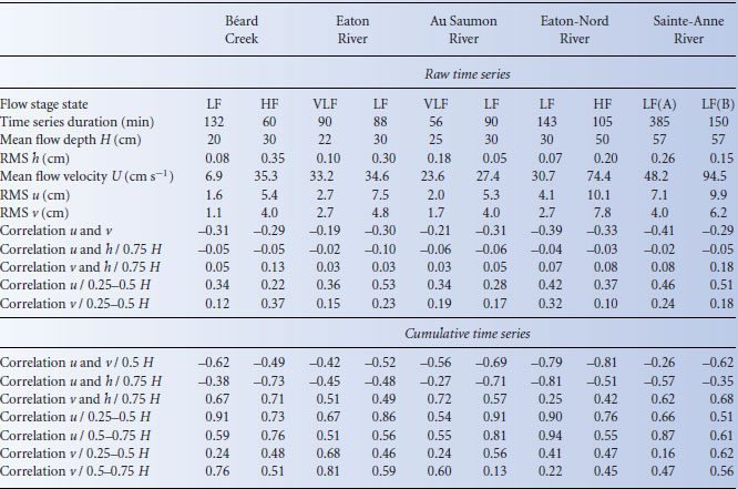
The instruments were mounted on an aluminum frame of dimensions 1.5 m by 1.5 m to allow stable long-term measurements. The frame was located in the thalweg at the downstream end of a pool where the flow was locally uniform with no drastic bed elevation variations or protruding obstacles upstream of the instruments (Figure 17.1). Time series were sampled for as long as possible given the river scale, the stability of the flow stage and the practical constraints such as the time available once the instrumental set-up was completed. The duration of the time series and the principal flow characteristics are presented in Table 17.2. The field sampling was completed by a pebble count of 300 particles and by a total station survey covering two riffle-pool units upstream of the measurement location except for the two reaches of the Sainte-Anne River (Figure 17.1). For these reaches, only the first riffle-pool unit was surveyed due to time constraints. The second riffle-pool unit was measured using a tape. All the morphological dimensions given in Table 17.1 were extracted from the interpolation of the total station surveys presented in Figure 17.1. To distinguish the mean flow depth H at the exact location of the measurements, we use Y for the average reach flow depth, YR for the riffle flow depth and YP for the pool flow depth.
Table 17.2 Field time series characteristics (shown for 0.5H except when mentioned).
17.2.2 Data analysis
Before proceeding to further analysis, the ECM signals were visually inspected to identify discontinuities and anomalous spikes, most often associated with leaves or other debris hitting the probes. Following data inspection, raw signals were defiltered to remove the effect of the analog R/C filter in the ECM measurements according to the recommendations from Roy et al. (1997). Data spikes were removed using the procedure of Goring and Nikora (2002), and high-frequency electronic noise above the Nyquist frequency was filtered using a third-order Butterworth filter. The ultrasonic sensor time series were not processed extensively, except for data spikes larger than three times the standard deviation, which were replaced by linear interpolation using neighbouring data points. Finally, the stationarity of all time series was validated by testing if the slope of the linear regression between the flow height measurements and time was equal to 0. The time series were shortened as needed to obtain a zero slope (α = 0.01).
Identifying different length scales of flow structures from single point measurements implies the use of the Taylor's hypothesis of frozen turbulence in order to represent temporal measurements as if observed in a spatial domain. This technique has led, in particular, to the discovery of the VLSM or superstructures described in the introduction. However, there is still some contention about the validity of Taylor's hypothesis over large distances. When comparing point velocity measurements, constructed by applying Taylor's hypothesis, with spatial PIV measurements, Dennis and Nickels (2008) found a high correlation for the large-scale structures between the two fields after filtering out the small-scale structures. Even though their experiment covered a streamwise distance of only 6δ, this suggests that Taylor's hypothesis can be used effectively if it is only the large scales that are of interest as the small structures deform too rapidly. For our data, applying Taylor's hypothesis to flow scales as large as the pool spacing may lead to approximate results. Nevertheless, it seems sensible to postulate that as CFS increase in scale their persistence in time and space also increases and that the very large CFS are more likely to be decaying as they pass the probe. Thus, the scales determined using Taylor's hypothesis, even though they may be inaccurate, can be considered as lower bound estimates, which reinforces the conclusion that large CFS exist.
To detect various scales of flow structures embedded in a velocity signal, spectral analysis is often the preferred method. In Marquis and Roy (2011), the time series were too short to use spectral analysis as the pulsations repeated only two to four times in the series. We detected the flow pulsations by using alternative analysis. In this study, we measured much longer velocity time series, from 56 to 385 min, in order to observe a larger number of pulsation cycles and in the hope of using spectral analysis to detect even the largest scales of flow motion. Supposing that the largest expected scale of CFS is equal to the pool spacing of the reach where velocity time series were measured, between 10 and 45 cycles could be detected in the time series, except for the HF measurements at Béard Creek where 100 cycles can potentially be detected. Figure 17.2 presents the premultiplied power spectrum of the streamwise velocity at 0.5H for the HF at Béard Creek. In premultiplied power spectra, equal areas under the curves correspond to equal energies, which is useful to interpret the larger scales of flow motions. In Figure 17.2, peaks are visible at scales of LSM (2-6H) and VLSM (10-20H). But, even though VLSM are detected, their energy is much smaller than LSM, probably because they are less periodic, but it does confirms the existence of such long structures in natural river flows. These results are representative of all the premultiplied power spectra of the time series measured in the other reaches (not shown here).
Figure 17.2 Premultiplied power spectrum of the streamwise velocity at 0.5H at Béard Creek HF. Taylor's hypothesis of frozen turbulence was used to estimate the wavelength λ from the frequencies f of the spectral analysis, assuming that the convection velocity equals the mean velocity U (λ = U/f). The spectral density Φ is multiplied by the wavenumber k where k = 2πf and made nondimensional using friction velocity u*. The spectrum is averaged from spectra estimated on 50 segments of the time series.
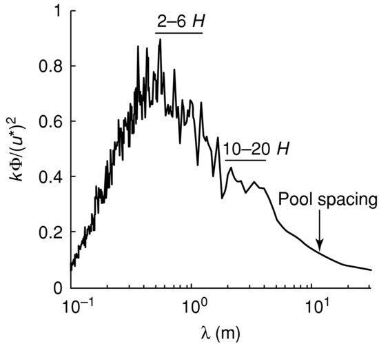
Even though the time series used in Figure 17.2 is the one where we should see most clearly the largest scales of flow motion because it is the one with the greater number of possible observable pulsation cycles; there are no visible peaks at wave lengths larger than 20H, which corresponds to only half of Béard Creek pool spacing. Similar results were obtained for all studied reaches and no characteristic scales larger than about 20H can be observed in the spectra. This lack of detection of the very-large scales of flow motion by the spectral analysis may be because they are not present in the time series, but it can also be due to other reasons:
- For some of the time series, there might be not enough cycles, or their lengths are too variable to obtain clear wavelength detection by a spectral analysis.
- The deformation of the structures as they evolve through time results in an underestimation of their length by spectral analysis (Kim and Adrian, 1999).
- The potential meandering of the very large structures may lead to a misinterpretation of length scales from one-dimensional energy spectra (Hutchins and Marusic, 2007).
- Even if there is no meandering, multiple and overlapping scale distributions may contaminate the final spectral estimate (Hutchins and Marusic, 2007).
Spectral analysis does not therefore seem to be appropriate to detect very large-scale flow structures from single point measurements using Taylor's hypothesis of frozen turbulence. We will use several nontraditional approaches to detect the presence or the absence of flow pulsations within the velocity signal. Figure 17.3a shows an example of 30 minutes of the time series measured at 0.5H for low flow-stage conditions in Béard Creek. There are no obvious low frequency oscillations in the raw streamwise or vertical velocity components of the flow and in the flow depth fluctuations as the high-frequency variations display large amplitude. To detect the low frequency oscillations embedded in the signal, the effect of the small structures should be removed. This is consistent with the study of Dennis and Nickels (2008) where the small turbulent structures were responsible for loss of correlation between the Taylor field and the spatial velocity field. To do so, we used two different types of time series transformation: (i) cumulative departures from the mean analysis and (ii) smoothed velocity and turbulent quantities time series. Using two different types of analysis should strengthen our conclusions if the results converge. To make sure that low-frequency oscillations detected in the time series are not artefacts of the analyses, we applied the same analysis to a set of random time series. Those time series were generated using normal distributions and the parameters (mean and standard deviation) of u, v and h time series for each measured reach and flow stage.
Figure 17.3 Raw time series (a) and transformed times series (b to e) for the low flow stage measurements at Béard Creek and a comparison with a random time series generated from Béard Creek low flow parameters. Only measurements at 0.5H are presented.
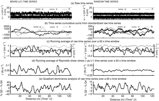
Cumulative departure analysis has long been used for hydrological and meteorological data analysis and for aquifer recharge evaluation (Kraus, 1956; Weber and Stewart, 2004). When used on normally distributed data, i.e. the median equals about the mean, it is a tool that offers the advantage of detecting shifts in the mean of the time series and changes in trends in the data (Buishand, 1982). The cumulative sum time series are generated by summing successively the residuals from the mean from the first time lag to the last. This impels the cumulative time series to begin and finish at the zero value. Therefore, by cumulating the sums of the deviations of the streamwise (u′) and vertical (v′) velocity components and of the water depth fluctuations (h′), it is possible to observe low-frequency oscillations while the high-frequency fluctuations are damped as shown by Marquis and Roy (2011). There are periods when positive fluctuations are more frequent or stronger than negative fluctuations (or vice versa) which results in a positive (or negative) trend of the cumulative sum of the time series fluctuations (Figure 17.3b). It is the slope of a cumulative curve that is of interest and not its position compared to the zero line. For the streamwise velocity, an upslope curve means that there is an excess in positive velocity fluctuations and that the flow is generally accelerating. It is the opposite for a downslope. For example, at the very beginning of the plot for the Béard Creek time series (LF) in Figure 17.3b, there is no obvious trend as all the curves stay near zero but, after a short while, the streamwise velocity fluctuations tend to be globally positive as the cumulative curve slope is positive. But then, the slope of the curve returns to a null value, meaning that there is no preferential trend in streamwise fluctuations during that period, even though the cumulative curve is high above the zero line.
Another way to damp the effect of high frequency fluctuations of the small-scale turbulent CFS is to smooth the signal, as Dennis and Nickels (2008) did. There are multiple smoothing methods available but we will use only the simplest one, the running average, which will detect the largest fluctuations if they exist. We used a moving window of 60 s to obtain the smoothed series of u′, v′ and h′ in Figure 17.3c. The choice of the length of the window is based on the fact that the window should be large in relation to the turbulent scale (a few seconds) and be smaller than the smallest expected pulsation length in the data set with respect to our hypothesis concerning the potential control of the pool spacing on the pulsation length. By dividing the pool spacing of the river (Table 17.1) by mean flow velocity (Table 17.2), the expected pulsation durations are all longer than 60 s except for the high flow conditions at Béard Creek where the expected duration is 34 s. We evaluated the effect of using a moving time window of 30 s compared to one of 60 s on the estimation of the pulsation duration and there was no significant difference. We decided to use the 60 s time window for all the data sets because it is generally recognized (cf. Buffin-Belanger and Roy, 2005) that a sample of one minute is the minimum record length to obtain stable parameters to characterize river mean and turbulent flow properties.
The running average time series of u′ were used to calculate the length of the flow pulsations as it is for this component that the oscillations are the strongest (Figure 17.3) and also because previous studies on VLSM and superstructures primarily used the streamwise component of the flow. The U-level detection scheme (Luchik and Tiederman, 1987) applied to the running average time series of u′ was used to detect low- and high-speed pulsations. The detection scheme identifies high-speed structures when the running average time series is higher than the mean and low-speed structures when the averaged time series is lower than the mean. The duration of a pulsation was considered to be a complete cycle composed of successive low- and high-speed pulsations (Marquis and Roy, 2011). For each time series, we averaged all durations of the detected flow pulsations at all three heights to obtain a single value for each set of measurements. The average duration was multiplied by the mean flow velocity to obtain a ‘typical’ pulsation length. To appreciate the variability in pulsation lengths for the same time series, we also estimated the 25th and 75th percentiles of the distribution.
To illustrate the effect of the flow pulsations on the general characteristics of the flow and possibly on river processes such as sediment transport, we also calculated the running average time series with a moving time window of 60 s of the Reynolds shear stress (τ):
(17.1) 
where ρ is the water density of 1000 kg m−3 (Figure 17.3d). Finally, we also estimated over moving time windows of 60 s the duration imbalance between the two dominant macroturbulent LSM, ejection-like low-speed wedges and sweep-like high-speed wedges, by using the quadrant detection technique (Willmarth and Lu, 1972). We focused on these CFS as they are known to be responsible for most of the momentum exchange between the inner and outer regions of the flow in the turbulent boundary layer (Kline et al., 1967). Ejection-like structures (quadrant 2, Q2) correspond to u′ < 0 and v′ > 0 while sweeplike structures (quadrant 4, Q4) correspond to u′ > 0 and v′ < 0. Over a given 60 s window, we detected the structures and subtracted the percentage of time occupied by sweep-like structures from the percentage of time occupied by ejection-like structures. This procedure allowed us to obtain a time series of the type of CFS dominance over time (Figure 17.3e).
17.3 Results
17.3.1 Time series characteristics
The velocity time series measured in the field are comparable to other steady uniform fully developed turbulent flows in gravel-bed rivers (e.g. Kirkbride and Ferguson, 1995; Buffin-Belanger et al., 2000; Roy et al., 2004). In general, the u and v components at the same flow height are negatively correlated while each velocity component measured at different depths is positively correlated. This indicates the presence of high- and low-speed wedge LSM occupying the entire flow depth and the dominance of ejection-like and sweeplike CFS in the flow. The correlations between the water height fluctuations and the two velocity components are weak even though the signs of the correlation coefficients may be what one would expect: an inverse relation between u and h and a positive relation between v and h. These relations imply that when there is a low-speed LSM, the water surface tends to bulge with a dominant vertical velocity toward the surface and when there is a high-speed LSM, water height tends to decrease corresponding to a vertical velocity oriented toward the bed. When examining the correlations between the cumulative sums of the fluctuations in the time series, the same characteristics as those observed from the analyses of the raw velocity time series are revealed but with higher correlation coefficients, which confirms the existence of a range of scales of similar CFS (Table 17.2). The pairwise correlation coefficients between the streamwise velocity components measured at different flow depths range between 0.51 and 0.94. The correlations between the cumulative fluctuations time series of u and h are strongly negative while those of v and h are strongly positive. This confirms that the flow pulsations occupy the entire flow depth.
17.3.2 Flow pulsation detection
Figure 17.3 presents two examples of 30-minutes duration, the first from data measured at Béard Creek at low flow and the second from a random time series with similar mean and standard deviation flow velocity. The horizontal axes of the plots in Figure 17.3 represent distances estimated using the Taylor frozen turbulence hypothesis. The substitution of time by space allows an appreciation of the length scales considered here and their comparison to the stream morphology. From the typical instantaneous velocity time series (Figure 17.3a), low frequency oscillations are revealed in the streamwise and vertical velocity and in the water height signals from both the cumulative sum of the fluctuations and the moving average analyses (Figure 17.3b, c). The low-frequency oscillations are several metres long, can last from several seconds up to a few minutes and correspond to flow pulsations that are detected in both velocity components. These pulsations have a direct influence on the variability of the Reynolds shear stress, which also exhibits well-defined and quite regular low-frequency cycles in synchronicity with the velocity oscillations (Figure 17.3d). The low frequency pulsations in the streamwise and vertical components also result in marked fluctuations of the relative proportions of ejections and sweeps (Figure 17.2e). The two examples shown in Figure 17.3 are typical of all field and random velocity and water height time series.
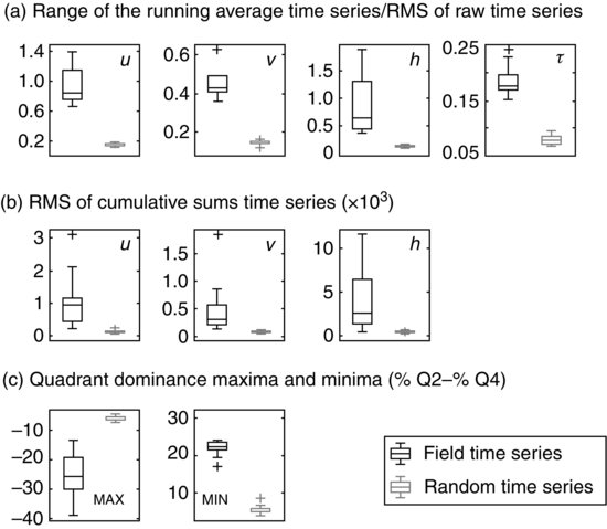
What distinguishes the random time series from the field time series is the amplitude of the low frequency oscillations. The amplitude of the low-frequency oscillations embedded in the cumulative sums and running average time series is much greater for Béard Creek time series compared to the random time series, even though the two data sets have similar mean and standard deviation of velocity (Figure 17.3b–e). Extending this comparison to the whole data set, the amplitude of the flow pulsations for the streamwise and vertical velocity components, the water height and the Reynolds shear stress is much greater in the field data than in the equivalent random time series (Figure 17.4a). Large differences between field and random data sets also occur for standard deviation (RMS) of cumulative sums and for maxima and minima defining the imbalance between ejections and sweeps (Figure 17.4b,c). Applying the same procedures and analyses to random time series to assess the amplitude of the resulting signals clearly shows that the flow pulsations detected in the field time series are not artefacts of our analyses. The amplitude of the random time series is much smaller than the amplitude of field data, showing that low frequency oscillations truly exist in the measured river flows (Figure 17.4). An examination of the amplitudes of the cumulative sums and running average time series of u, v and h also shows that the coherent organization of the flow is strongest in the streamwise velocity and the water height compared to the vertical velocity (Figure 17.4).
Figure 17.4 Comparisons of the flow pulsation amplitudes for different analyses between the field time series and random time series (generated based on the characteristics of the field time series).
17.3.3 Flow pulsation scalings
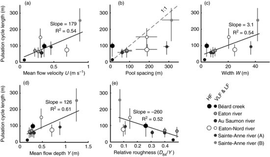
Figure 17.5 presents the relations between average pulsation length and the main flow and morphological variables. Average flow-pulsations length varies from 10 to 300 m. Their range of variation is relatively large and covers several metres for one set of time series as illustrated in Figure 17.5. It may represent various stages of flow pulsation formation, the largest one being detected on a few occasions but probably representing the maximal extension of the phenomena. This aperiodicity is probably the main reason why flow pulsations could not be detected from spectral analysis. Figure 17.5a shows flow pulsation length against mean flow velocity. A strong correlation here would suggest that a self-organization process might contribute to the flow pulsations formation. Because of the use the mean flow velocity as the convection velocity for the application of the Taylor hypothesis, a spurious correlation should be present here. The relation is relatively strong (R2 = 0.54) but this is mainly influenced by data for the Sainte-Anne River B. Without this outlier, the relationship between the average flow pulsation length and the mean flow velocity would be much weaker and not significant. Figure 17.5b presents the scaling between flow pulsation length and pool spacing. According to our hypothesis, most of the points should fall on the 1:1 line, which is the case for 70% of the points when considering the upper range of the flow pulsation lengths. Three sets of flow pulsation measurements fall outside the 1:1 line, among which two were sampled during high flow conditions. This weakens our hypothesis and hints at the fact that other morphological features of the selected reaches may control the length of the flow pulsations. Pulsation length does scale with the channel width occupied by the flow and with the flow depth but the relations display some scatter (Figure 17.5c,d). Figure 17.5e shows that as the relative submergence of isolated roughness elements (D84 /H) increases, flow pulsation length decreases. The scalings presented in Figure 17.5 do not allow for a simple confirmation of the morphological hypothesis suggesting that pool spacing controls pulsation length but the results provide a basis for discussing the mechanisms that could explain the origin of the pulsations.
Figure 17.5 Relations between the pulsation cycle lengths measured in the field and (a) the mean flow velocity (b) the pool spacing, (c) the channel flow width, (d) the mean flow depth of the reach and (e) the relative roughness of the reach. The grey vertical lines represent the range of values between the percentiles 25 and 75 of the pulsation lengths. The horizontal grey lines in (b) represent the range of pool spacing upstream of the measurement point.
17.4 Discussion
In this chapter we identified low-frequency oscillations, which we have called flow pulsations, in the streamwise and vertical instantaneous velocity signals and in the water-height fluctuations. The flow pulsations identified here are larger than any reported in the literature for flows over a static bed as their length is around one hundred times the flow depth. The only low-frequency oscillations of similar scales were reported for a flow over mobile bedforms in a river by Dinehart (1999) and in a flume by Singh et al. (2010). Those oscillations are different as they relate to local flow depth variation and not to the coherent organization of flow structures. Our first objective was to show that such long-cycle flow pulsations are characteristic features of shallow flows over rough river beds. Our measurements of long velocity time series in the field present low frequency oscillations (i.e. flow pulsations) embedded in the signal. Because spectral analysis failed to identify the largest scales of flow motion (Figure 17.2) and because the use of the Taylor hypothesis may be inaccurate, we used two different types of analysis to reveal the presence of the pulsations (Figure 17.3). In the light of the results, the deformation of the structures as they convect downstream may lead to a wide range of detected pulsation lengths (Figure 17.5). The apparent nonperiodicity of the pulsations probably prevents the detection of the structures by spectral analysis. It is not possible to state if the flow pulsations are truly aperiodic or if they appear as such as a result of using Taylor's hypothesis in the different analyses (cumulative departures and running average). The comparison between the field flow pulsation amplitudes and those of randomly generated time series confirms that the detection of flow pulsations is not an artefact of the analyses (Figure 17.4). Flow pulsations seem to be characteristic CFS in shallow gravel-bed river flows.
Our second objective was to investigate the possible origin of the flow pulsations with respect to two alternative hypotheses: self-organization of macroturbulent LSM into larger flow pulsations and the morphological control on the pulsation lengths. One of the main schools of thought in the study of turbulence seeks to break the complex, multiscaled, random fields of coherent flow motion down into more elementary organized motions (Adrian, 2007). Many have argued that individual turbulent CFS are the building blocks that form larger coherent structures such as VLSM or superstructures with lengths up to 20δ (Hutchins and Marusic, 2007). Adrian (2007) questioned the maximal extent of the build-up of small structures into larger ones. Even though the scale of the flow pulsations is larger than that of VLSM, we postulate that these two phenomena are similar. Therefore, the pulsations described in this paper could very well be a bottom-up process as they have characteristics similar to the typical macroturbulent LSM. They occupy the entire flow depth and exhibit a negative correlation between the streamwise and vertical velocity component (Table 17.2). Also, they exhibit a mild scaling with mean flow velocity, which could be typical of macroturbulent LSM (Shvidchenko and Pender, 2001). But, it is not possible to discern conclusively from the data here whether flow pulsations indeed result from progressive amalgamation of small-scale turbulent structures or from being just a chance alignment of the LSM as suggested by Dennis and Nickels (2011). The fact that the pulsations can be caused by a random alignment of similar LSM could be supported by the wide range of lengths and aperiodic occurrences, which tend to suggest that there is no outer mechanism controlling their length (see error bars in Figure 17.5). But, the scaling of their median length with various morphological characteristics of the channel strongly suggests that the boundary controls, at least partly, the scale of the flow pulsations in the sampled reaches.
The hypothesis of a pool spacing control on the pulsation length, as proposed by Marquis and Roy (2011), implies that, for a given river, pulsation length would remain constant for different flow stages. In Figure 17.5b, even if most of the data points (7 out of 10) are close to the 1:1 line, there are three outliers that impede unambiguous confirmation of pool spacing control on pulsation lengths. We have explored other morphological variables and the best fit was with the relative submergence of isolated roughness elements. Even though these elements are known to have only a local effect on the flow (Lamarre and Roy, 2005; Lacey and Roy, 2007), it is plausible to assume that, when local roughness elements protrude relatively high in the flow, there is less chance that long flow structures form and travel downstream. In other words, they limit the maximal extent of the flow pulsations. But isolated roughness elements also increase the turbulence intensity of the flow (e.g. Buffin-Belanger and Roy, 1998) so they may contribute to the generation of the pulsations.
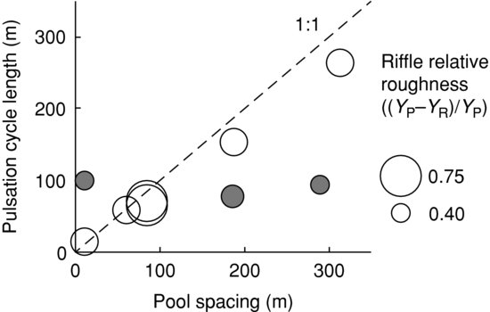
These results also lead us to consider the relative submergence of the riffles defined as (YR−YP)/YP. Redrawing Figure 17.5b, the relation between pulsation length and pool spacing, with the data points that are proportional in size to the riffle relative submergence (Figure 17.6) reveals that the three outliers (in shaded grey) have the smallest relative riffle roughness (around 0.4). Two of these points correspond to high flow stages measured at Béard Creek and the Eaton-Nord River. The third point is the low flow stage set of measurements at Sainte-Anne River A. This site is an elongated pool without marked flow expansion at the entrance or flow contraction at the exit (Figure 17.1). All measurements taken at very low and low flow stages have pulsation lengths that scale with pool spacing. The riffle relative roughness could act as a control of the flow pulsation cycle length perhaps by a process akin to a fill and spill of the pool associated with the flow contraction or choking over the riffle. When the flow passes over the riffle, there might be a backwater effect (on a millimetre scale) that is released on a regular or pseudoperiodic basis and the surge would therefore control the frequency of the flow pulsations. This control would also be confirmed by the occurrence of low-frequency oscillations in water surface height fluctuations that correlate with the streamwise and vertical velocity pulsations. The constriction of the flow imposed when riffle submergence is high might have an effect on the flow surface which in turn affects the velocity fields. This hypothesis implies that the flow pulsations would be as wide as the channel, a statement that we cannot confirm from our measurements. Our measurements of the water surface fluctuations also support Levi's hypothesis (1983) concerning the outer control of coherent flow structures generation by travelling surface waves.
Figure 17.6 Relation between the pulsation cycle lengths measured in the field and the pool spacing. The size of the data points is proportional to the riffle relative roughness. The outliers are identified by grey circles instead of white.
17.5 Implications and conclusions
The results do not confirm whether the flow pulsations originate from a bottom-up process, a top-down process or a mixture of both. We propose that flow pulsations tend to exist inherently in a flow above a rough bed but that there is a positive feedback mechanism through the relative submergence of isolated roughness elements and of riffles as it is combined with pool spacing that may reinforce their structure and modulate their length. This mixture of processes to explain the origin of flow pulsation also highlights the possibility that the transition from small-scale turbulent phenomena to the channel boundary conditioning of coherent flow structures is probably continuous. Furthermore, different mechanisms may produce flow structures with similar scales, which may be a source of confusion when trying to tackle CFS-generating processes as exemplified in this chapter. Despite the focus of the discussion on the origin of the flow pulsations, the simple fact that such pulsations exist and are ubiquitous in shallow flows over gravel beds is a major contribution toward understanding fluvial processes in general. In particular, bedload transport is known to have a pulsating behaviour where the peaks and troughs in transport rates are not correlated to flow variables such as discharge or stream power (e.g. Reid et al., 1985; Gomez et al., 1989). These pulses are often associated with bedload sheets travelling downstream (Whiting et al., 1988) but their formation process is not yet fully understood (Recking et al., 2009).
On the other hand, low-frequency velocity oscillations were correlated to migration of bedforms during a high flow stage in a gravel-bed river (Dinehart, 1999; Singh et al., 2010). Here, we have shown that low-frequency oscillations, the flow pulsations, exist during steady flows over static bedforms. It is possible that flow pulsations interact with bedload transport to create pulses of grains travelling downstream. Furthermore, flow pulsations have an impact on variables that contribute to individual grain entrainment. We have shown that the Reynolds shear stress and the quadrant dominance through time also exhibit low frequency oscillations with large departures from the mean values. In light of these different findings for flows with and without active bedload transport, it is sensible to hypothesize that the bedforms and the flow pulsations interact in a retroaction cycle. While static large bedforms could control the scale of flow pulsations at low flows, flow pulsations could in turn control bedforms migration at high flows. A better understanding of flow pulsation scalings could allow us to potentially relate these CFS to the scale of bedload pulses, which have similar length scales.
17.6 Acknowledgements
The authors would like to thank Rachel Thériault and Claude Gibeault for their help in the field. We also acknowledge the financial support of National Science and Engineering Council (NSERC) and the Canadian Foundation for Innovation (CFI).
References
Adrian, R.J. (2007) Hairpin vortex organization in wall turbulence. Physics of Fluids 19, 041301. DOI: 10.1063/1.2717527.
Adrian, R.J., Meinhart, C.D. and Tomkins, C.D. (2000) Vortex organization in the outer region of the turbulent boundary layer. Journal of Fluid Mechanics 422, 1–54.
Bonacci, O. (1979) Influence of turbulence on the accuracy of discharge measurements in natural streamflows. Journal of Hydrology 42, 347–367.
Buffin-Belanger, T. and Roy, A.G. (1998) Effects of a pebble cluster on the turbulent structure of a depth-limited flow in a gravel-bed river. Geomorphology 25, 249–267.
Buffin-Belanger, T. and Roy, A.G. (2005) 1 min in the life of a river: selecting the optimal record length for the measurement of turbulence in fluvial boundary layers. Geomorphology 68, 77–94.
Buffin-Belanger, T., Roy, A.G. and Kirkbride, A.D. (2000) On large-scale flow structures in a gravel-bed river. Geomorphology 32, 417–435.
Buishand, T.A. (1982) Some methods for testing the homogeneity of rainfall records. Journal of Hydrology 58, 11–27.
Dement'ev, V.V. (1962) Investigations of pulsation of velocities of flow of mountain streams and its effect on the accuracy of discharge measurements. Soviet Hydrology: Selected Papers 1, 588–623.
Dennis, D J.C. and Nickels, T.B. (2008) On the limitations of Taylor's hypothesis in constructing long structures in a turbulent boundary layer. Journal of Fluid Mechanics 614, 197–206.
Dennis, D.J.C. and Nickels, T.B. (2011) Experimental measurement of large-scale three-dimensional structures in a turbulent boundary layer. Part 2. Long structures. Journal of Fluid Mechanics 673, 218–244.
Dinehart, R.L. (1999) Correlative velocity fluctuations over a gravel river bed. Water Resources Research 35, 569–582.
Falco, R.E. (1977) Coherent motion in the outer region of turbulent boundary layers. Physics of Fluids 20, s124–s132.
Ganapathisubramani, B., Longmire, E.K. and Marusic, I. (2003) Characteristics of vortex packets in turbulent boundary layers. Journal of Fluid Mechanics 478, 35–46.
Gomez, B., Naff, R.L. and Hubbell, D.W. (1989) Temporal variations in bedload transport rates associated with the migration of bedforms. Earth Surface Processes and Landforms 14, 135–156.
Goring, D.G. and Nikora, V.I. (2002) Despiking acoustic doppler velocimeter data. Journal of Hydraulic Engineering 128, 117–126.
Hutchins, N. and Marusic, I. (2007) Evidence of very long meandering features in the logarithmic region of turbulent boundary layers. Journal of Fluid Mechanics 579, 1–28.
Kim, K.C. and Adrian, R.J. (1999) Very large-scale motion in the outer layer. Physics of Fluids 11, 417–422.
Kirkbride, A.D. and Ferguson, R. (1995) Turbulent flow structure in a gravel-bed river: Markov chain analysis of the fluctuating velocity profile. Earth Surface Processes and Landforms 20, 721–733.
Kline, S.J., Reynolds, W.C., Schraub, F.A. and Runstadler, P.W. (1967) The structure of turbulent boundary layers. Journal of Fluid Mechanics 30, 741–773.
Kraus, E.B. (1956) Graphs of cumulative residuals. Quarterly Journal of the Royal Meteorological Society 82, 96–98.
Lacey, R.W.J. and Roy, A.G. (2007) A comparative study of the turbulent flow field with and without a pebble cluster in a gravel bed river. Water Resources Research 43, W05502. DOI: 10.1029/2006WR005027.
Lamarre, H. and Roy, A.G. (2005) Reach scale variability of turbulent flow characteristics in a gravel-bed river. Geomorphology 68, 95–113.
Levi, E. (1983) Oscillatory model for wall-bounded turbulence. Journal of Engineering Mechanics 109, 728–740.
Liu, Z., Adrian, R.J. and Hanratty, T.J. (2001) Large-scale modes of turbulent channel flow: transport and structure. Journal of Fluid Mechanics 448, 53–80.
Luchik, T.S. and Tiederman, W.G. (1987) Timescale and structure of ejections and bursts in turbulent channel flows. Journal of Fluid Mechanics 174, 529–552.
Marquis, G.A. and Roy, A.G. (2006) Effect of flow depth and velocity on the scales of macroturbulent structures in gravel-bed rivers. Geophysical Research Letters 33, L24406. DOI: 10.1029/2006GL028420.
Marquis, G.A. and Roy, A.G. (2011) Bridging the gap between turbulence and larger scales of flow motions in rivers. Earth Surface Processes and Landforms 36, 563–568.
Matthes, G.H. (1947) Macroturbulence in natural stream flow. Transactions of the American Geophysical Union 28, 255–265.
Nakagawa, H. and Nezu, I. (1981) Structure of space-time correlations of bursting phenomena in an open-channel flow. Journal of Fluid Mechanics 104, 1–43.
Nezu, I. and Nakagawa, H. (1993) Turbulence in Open-Channel Flows, A.A.Balkema, Rotterdam.
Nikora, V. (2007) Hydrodynamics of gravel-bed rivers: scale issues. In Gravel-Bed Rivers VI: From Process Understanding to River Restoration (eds H. Habersack, H. Piégay and M. Rinaldi). Elsevier, Amsterdam, pp. 61–81.
Recking, A., Frey, P., Paquier, A. and Belleudy, P. (2009) An experimental investigation of mechanisms involved in bed load sheet production and migration. Journal of Geophysical Research – Earth Surface 114, F03010. DOI: 10.1029/2008jf000990.
Reid, I., Frostick, L.E. and Layman, J.T. (1985) The incidence and nature of bedload transport during flood flows in coarse-grained alluvial channels. Earth Surface Processes and Landforms 10, 33–44.
Roy, A.G., Biron, P.M. and Lapointe, M.F. (1997) Implications of low-pass filtering on power spectra and autocorrelation functions of turbulent velocity signals. Mathematical Geology 29, 653–668.
Roy, A.G., Buffin-Belanger, T., Lamarre, H. and Kirkbride, A.D. (2004) Size, shape and dynamics of large-scale turbulent flow structures in a gravel-bed river. Journal of Fluid Mechanics 500, 1–27.
Rood, K.M. (1980) Large Scale Flow Features in Some Gravel Bed Rivers. Master's thesis. Simon Fraser University, Burnaby.
Shvidchenko, A.B. and Pender, G. (2001) Macroturbulent structure of open-channel flow over gravel beds. Water Resources Research 37, 709–719.
Singh, A., Porté-Agel, F. and Foufoula-Georgiou, E. (2010) On the influence of gravel bed dynamics on velocity power spectra. Water Resources Research 46, W04509. DOI: 10.1029/2009wr008190.
Toh, S. and Itano, T. (2005) Interaction between a large-scale structure and near-wall structures in channel flow. Journal of Fluid Mechanics 524, 249–262.
Tomkins, C.D. and Adrian, R.J. (2003) Spanwise structure and scale growth in turbulent boundary layers. Journal of Fluid Mechanics 490, 37–74.
Weber, K. and Stewart, M. (2004) A critical analysis of the cumulative rainfall departure concept. Ground Water 42, 935–938.
Whiting, P.J., Dietrich, W.E., Leopold, L.B. et al. (1988) Bedload sheets in heterogeneous sediment. Geology 16, 105–108.
Willmarth, W.W. and Lu, S.S. (1972) Structure of the Reynolds stress near the wall. Journal of Fluid Mechanics 55, 65–92.
Zhou, J., Adrian, R.J., Balachandar, S. and Kendall, T.M. (1999) Mechanisms for generating coherent packets of hairpin vortices in channel flow. Journal of Fluid Mechanics 387, 353–396.