20
Turbulence Modulation by Suspended Sediment in a Zero Mean-Shear Geophysical Flow
ABSTRACT
The effects of suspended sediment transport on turbulent geophysical flows have long been debated in the literature. Yet there remains ambiguity in the results and in the interpretation of criteria commonly employed to discriminate the occurrence of turbulence modulation, especially in experimental open channel flows. To address some of these issues, the effects of suspended sediment on fluid turbulence were investigated using a standard mixing box where a single oscillating grid was placed near the floor of the apparatus. Flow conditions within the box for a given grid oscillation frequency were quantified using particle image velocimetry where fluorescent tracer particles were used to discriminate the fluid phase, and changes to these fluid flow conditions were carefully monitored as concentrations of quartz-density sediment spanning supply-limited to transport-limited suspensions were introduced. The effects of suspended sediment on the magnitude of fluid turbulence in this geophysical flow were clear and significant. As suspended-sediment loadings increased in concentration for a given oscillation frequency, the magnitude of the fluid turbulence within the mixing box decreased markedly and systematically. While both turbulence enhancement and suppression were observed simultaneously in the same flow field, the overall effect of the suspended sediment load was to decrease fluid turbulence, total kinetic energy, and the rate of energy dissipation. It is contended here that the reduction in turbulent kinetic energy in the flow was due to the transfer of this energy to the sediment in suspension. The empirical evidence presented here demonstrated unequivocally that fluid turbulence could be significantly reduced in the presence of suspended sediment, and these observations should be applicable to a wide range of sediment-laden geophysical flows.
20.1 Introduction
The effect of suspended sediment transport on turbulent geophysical flows, in general, and open channel flows in particular, has long been debated in the literature. While sediment entrainment and transport depend on the time-mean and turbulence fluctuations in velocity and their associated fluid forces (see reviews in Bridge and Bennett, 1992; Bennett et al., 1998), it is reasonable to suppose that the characteristics of the flow are, in turn, affected by the presence of sediment. Much of the debate in open channel flows has focused on time-averaged profiles of velocity and Reynolds stress, the value of von Kármán's coefficient, and the magnitude, characteristics, and vertical distributions of turbulence intensities, mixing lengths, and eddy diffusion coefficients (see reviews in Best et al., 1997; Muste et al., 2005), and specifically how these parameters are altered in the presence of a suspended sediment load.
Mechanisms proposed for turbulence modulation in geophysical flows laden with sediment have been recently summarized by Balachandar and Eaton (2010). For dilute suspensions, turbulence reduction or suppression has been linked to (a) the enhanced inertia and (b) effective viscosity of the particle-laden flow, and (c) the increased dissipation arising from particle drag. Conversely, turbulence enhancement has been linked to enhanced velocity fluctuations due to wake dynamics and vortex shedding, and buoyancy-induced instabilities due to density variation arising from preferential particle concentration.
In open channels, three parameters are often used to define and characterize the effects of suspended sediment on fluid turbulence. The first criterion suggests that when particle diameter D is much smaller than the most energetic eddy, taken here as the integral length scale of turbulence λ, the particle will follow the eddy for part of its transit time (Gore and Crowe, 1989). As such, a portion of the turbulent energy of the eddy is transformed into the kinetic energy of the particle (via a drag force), which reduces the turbulent energy of the fluid. When D is relatively larger, these particles will tend to create turbulence in their wakes near the scale of the most energetic eddy λ, and increase the total turbulent energy of the fluid. The critical threshold for the transition from turbulence suppression to turbulence enhancement occurs at  . The second criterion suggests that turbulence modulation by suspended sediment occurs because a slip velocity exists between the particle in transport and the carrier fluid. This slip velocity can be expressed in terms of a particle Reynolds number Rep (
 , where subscripts f and p refer to the fluid and particle, respectively, and ν is the kinematic viscosity of the sediment-laden flow). According to Hetsroni (1989), when the particle Reynolds number is relatively low (
 ), turbulence tends to be reduced in the presence of suspended sediment. Yet when the particle Reynolds number is relatively high (
 ), particles in transport will shed vortices, and this phenomenon tends to increase fluid turbulence. The third criterion suggests that turbulence modulation by suspended sediment occurs because there is a difference in the response times of the particle in transport and the carrier fluid. The ratio of the particle response time tp to the fluid response time tf is the Stokes number St. According to Elghobashi (1994), when St<1, the surface area of the particles increases for a given volumetric suspended sediment concentration and this causes the rate of turbulence dissipation to increase, whereas when St>1, the particle Reynolds number, Rep increases, which then leads to vortex shedding (
 ). Both Best et al. (1997) and Muste et al. (2005) applied these criteria to explain their experimental observations in sediment-laden open channel flows. The results, however, were met with varying success, and included (i) subtle, or negligible, rather than marked variations in velocity and turbulence signatures, (ii) both enhancement and suppression of fluid turbulence in the same flow, (iii) inconsistency in the effects of sediment on turbulent flow, and (iv) the recognition that these criteria may not effectively capture or explain, in mechanistic terms, the occurrence of turbulence modulation.
It is contended here that the experimental design to examine the effects of suspended sediment on fluid turbulence can be improved. First, it is imperative that the fluid and sediment phases within a sediment-laden turbulent flow be clearly and unambiguously discriminated, therefore removing the potential that such turbulent signatures are contaminated by the other phase. Second, it is imperative that the clear-water and sediment-laden flows are, in fact, hydrodynamically equivalent, thus removing any uncertainty about varying flow rates, boundary conditions, and energy gradients when sediment is introduced to the clear-water flow.
The current research programme sought to quantify the effects of suspended sediment on fluid turbulence in a geophysical flow by specifically addressing these two experimental challenges. First, particle image velocimetry (PIV) is employed to quantify the turbulent flow field, where laser-induced fluorescent tracer particles coupled with lens-mounted polarized filters ensured that only the characteristics of the fluid phase are captured. Second, a standard grid-mixing box is employed (e.g. Thompson and Turner, 1975), such that the oscillation frequency and stroke of the grid can be externally controlled and total flow depth can be maintained, all with great precision, rather than employing an open channel. While an oscillating grid in a mixing box is, by definition, a zero mean-shear flow, the transport and decay of fluid turbulence from the grid and the dissipation of this energy are analogous to a wide range of geophysical flows, including open channels (e.g. Hopfinger and Toly, 1976; Michallet and Mory, 2004). Thus, the objectives of the current chapter are: (i) to quantify the time-mean and turbulent flow field within a mixing box using clear-water conditions, and (ii) to quantify the variations in the time-mean and turbulence characteristics of the fluid phase in the presence of a range of suspended sediment grains sizes and concentrations, spanning supply-limited to transport-limited conditions. It will be shown that suspended sediment, even in rather dilute concentrations, can markedly alter fluid turbulence, and its overall effect is to suppress the magnitude of these turbulent signatures.
20.2 Methods
All experiments were performed in a polycarbonate mixing box 0.315 m wide and deep, and 0.393 m tall (Figure 20.1). An aluminum grid placed near the bottom of the box provided the source of turbulence, and this orthogonal grid consisted of ten 10 mm square bars with 50 mm centre-to-centre spacing. The grid was mounted from above to a rotating eccentric arm and controlled by an external motor. Grid stroke was 90 mm, and the speed of the motor was measured with an optical tachometer. In all tests, the box was filled with tap water to a depth of 0.292 m.
Figure 20.1 Schematic diagram of mixing box and photograph of box with the grid oscillating at f = 2.33 Hz in the presence of 1000 g of 350 to 400 μm diameter quartz-density sand.
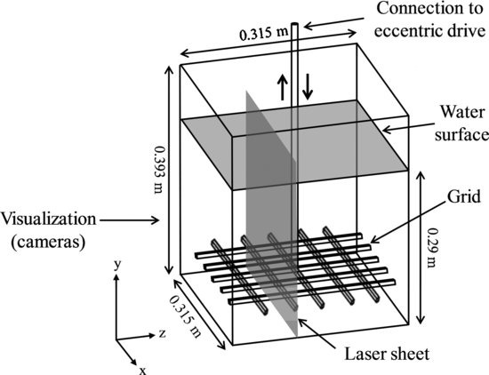
Particle image velocimetry was used to quantify all turbulence parameters within the box. This system comprised a dual-cavity 50 mJ Nd-YAG laser emitting 532 nm light and two 4 Mp cameras with 4 GB of RAM each. All data acquisition and synchronization was handled by an external timing hub, dedicated computer, and commercial software. Inside the box prior to experimentation, a dual-level 3D calibration target (0.27 m wide and 0.19 m tall) was placed at the apogee of the grid so that the target's surface was parallel with the plane of the laser. This captured image then was used to process the PIV data. The cameras were mounted off-axis to the plane of the laser (total angular difference of 16°), and only regions above the oscillating grid were recorded. For this study, paired images were collected at 40 to 80 Hz over a sampling period of several seconds (storage capacity in the cameras allowed saving approximately 512 images). The interrogation areas were 32 pixels (about 4 × 4 mm), and the central-difference adaptive correlation algorithm within the software was used to derive the 3D vector fields. The laser light sheet entered the box at 80 mm from the sidewall, and it was centred on the cross-bars of the grid rather than the nodes. Hollow glass spheres 20 to 50 μm in diameter and dyed with rhodamine B were used as fluid tracer particles, which fluoresced in the laser light sheet at a frequency greater than 570 nm (see Pedocchi et al., 2008). Polarizing filters (>570 nm) were placed on the camera lenses, thereby allowing only the fluorescent tracer particles to be captured (thus excluding emissions by the suspended sediment). The possibility of contamination of the PIV signal by the sand component, however, has not been tested. Each vector field comprised approximately 3000 vectors, and up to about 460 image pairs were used to derive time-averaged values of mean and turbulent velocities. All data reported here were actual measurements, and all time-averaged values had a minimum of 50 validated signals. The presence of suspended sediment did not measurably alter the quality of the measured data. Comparing the highest suspended sediment concentration data to the lowest, there is a 4% reduction in the number of vector positions quantified, while still retaining more than 106 actual velocity measurements for each time-averaged vector field.
Well sorted quartz-density sand, 250 to 300 μm in diameter, of varying concentration was used. Total added mass to the box varied from 100 to 1000 g at 100 g intervals, which was equivalent to a volumetric sediment concentration C0 (based on total water volume) ranging from 0.001302 to 0.013020. Volumetric suspended sediment concentrations C were collected at-a-point in the box using a siphon sampler. Both the volume of water and sediment removed after each sample extraction were replaced by equivalent amounts. These samples were decanted and the sediment oven-dried to determine total mass.
20.3 Results
The experimental data presented below will illustrate how turbulence is modulated by suspended sediment within a zero mean-shear flow. These data include variations in the volumetric suspended sediment concentration within the box as a function of total concentration and vertical height, the time-mean and turbulent flow field using clear-water conditions, and the variation of select flow parameters with increasing sediment concentration.
20.3.1 Variations in suspended sediment concentration
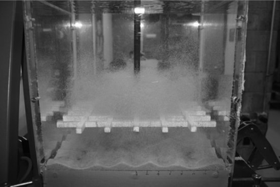
It is critical to determine the relationship between grid oscillation frequency f and volumetric suspended sediment concentration C, as normalized by the total volumetric sediment concentration in the box C0. For varying heights, y, above the grid apogee (y = 0), as normalized by total flow depth, d = 0.20, above this datum, and for a given oscillation frequency f, at-a-point values of C using 250 to 300 μm diameter sediment show that these concentrations reach asymptotic values at slightly different input concentrations, C0 (Figure 20.2a). If the input of additional sediment, C0, can affect the observed concentration, C, at-a-point, then this sediment suspension condition is deemed supply-limited even though some sediment could remain on the bottom of the box. If the input of additional sediment, C0, does not affect the observed concentration, C, at-a-point, then this sediment suspension condition is deemed transport-limited, and much sediment was observed on the bottom of the box (Figure 20.1).
Figure 20.2 Using f = 2.33 Hz, variations in volumetric suspended sediment concentration (a) at-a-point at a given y/d within the mixing box for a range of C0, and (b) as a function of y/d for two input concentrations C0 using 250 to 300 μm diameter quartz-density sand. Symbols represent two sets of measurements.
This distinction between supply-limited and transport-limited sediment suspensions within this zero mean-shear geophysical flow can be demonstrated by plotting C/C0 as a function of relative height in the box, y/d. Figure 20.2b shows that C/C0 remains fairly constant with distance from the grid when C0 = 0.00263, whereas when C0 = 0.00903, C/C0 remains fairly constant very near the grid (y/d<0.4), but decreases significantly with distance away from the grid (y/d>0.4). Thus for f = 2.33 Hz and particle sizes of 250 to 300 μm, suspended sediment is well mixed and supply limited when C0 = 0.00263, but displays a strong vertical gradient and is transport limited when C0 = 0.00903 (Figure 20.2b). Similar results have been obtained using other grain-size populations (Hou, 2011). It will be demonstrated here that sediment concentration can affect the modulation of fluid turbulence.
20.3.2 Time-mean and turbulent flow using clear-water conditions
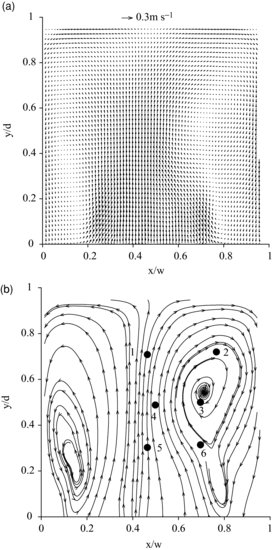
While the mixing box has no mean flow, oscillation of the grid does create a secondary circulation pattern. The time-mean 2D vectors (in the cross-stream x and vertical y directions; the transverse z velocity component is not shown here) and select streamlines for the clear-water conditions and f = 2.33 Hz are shown in Figure 20.3. Here, x/w is the relative distance across the box and w is the box width. It is well-known that an oscillating grid generates quasi-steady jet flow very close to each grid bar (Thompson and Turner, 1975). Above the grid, these jets interact and break down to create advecting turbulence whose magnitude decays with distance from the grid, as further modulated by the grid mesh spacing, oscillation frequency, and stroke (Hopfinger and Toly, 1976). For all tests conducted, flow within this plane of the mixing box is characterized by two large convection cells, and the largest magnitude secondary flow velocities are located in the centre of the field and are vertically oriented. Two counter-rotating convection cells bound this central flow region, returning fluid to the bottom of the tank along the box sidewalls. Secondary circulation within mixing boxes has been noted by others (Dohan and Sutherland, 2002; McKenna and McGillis, 2004), even though these apparatuses have been described as having a zero mean-shear flow. While the secondary circulation pattern observed here was not anticipated, its pattern does affect the distribution of flow velocity and turbulence.
Figure 20.3 Time-averaged 2D flow vectors (a) and select streamlines (b) within the mixing box for clear-water conditions using f = 2.33 Hz. The numbers refers to locations where autocorrelation analysis is applied.
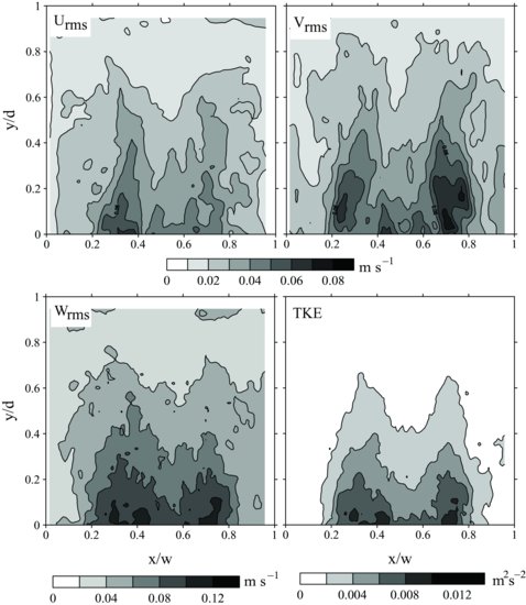
Turbulence parameters for the clear-water flow conditions can be defined as follows. Figure 20.4 shows contour maps of the root-mean-square of the cross-stream u (x-axis; Urms), vertical v (y-axis; Vrms) and transverse w components (z-axis; Wrms), defined as
(20.1) 
and the turbulent kinetic energy (TKE), defined as
(20.2) 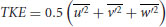
where u, v, and w are the instantaneous velocities at-a-point,  ,
,  , and
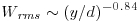
, and  , and the overbar represents an at-a-point time average. The distributions of turbulent velocities within the mixing box are in close association with distance from the grid and co-located with the highest magnitude velocity within the central portion of the convecting flow field. Regions of relatively low turbulence also occur along the sides of the box, where downward-directed flow velocities of the convection cells are located. As noted by Hou (2011), the decay of spatially-averaged turbulent velocities and kinetic energy with distance from the grid for the mixing box used here conforms reasonably well to expected relationships (Hopfinger and Toly, 1976):
 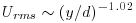 ;
; 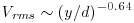 ;
;  ; and
; and 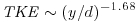 .
.
Figure 20.4 Contour plots of the root-mean-square of the u, v, and w component flow velocities and turbulent kinetic energy within the mixing box for clear-water conditions shown as a function of height above the grid using a grid oscillation frequency of 2.33 Hz.
20.3.3 Sediment-laden versus clear-water turbulent flow conditions
Relative changes of the turbulence parameters as observed in the sediment-laden flow conditions, compared with the clear-water results, were used to demonstrate the effects of suspended sediment on the turbulent flow field (fluid phase only). Only select examples of the time-mean and turbulent flow parameters for all sediment-laden conditions are shown here to illustrate these effects. The conditions include the 250 to 300 μm diameter sediment with f = 2.33 Hz and two input sediment loadings, C0 = 0.00263 and C0 = 0.00903, which represent supply-limited and transport-limited conditions, respectively. For comparative purposes, a normalized percentage difference (% difference) between the clear-water and sediment-laden conditions for the root-mean-square velocities and turbulent kinetic energy values can be defined simply as:
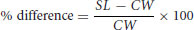
where SL and CW refer to the sediment-laden and clear-water flow parameter in question, respectively (thus allowing values to exceed ±100%).
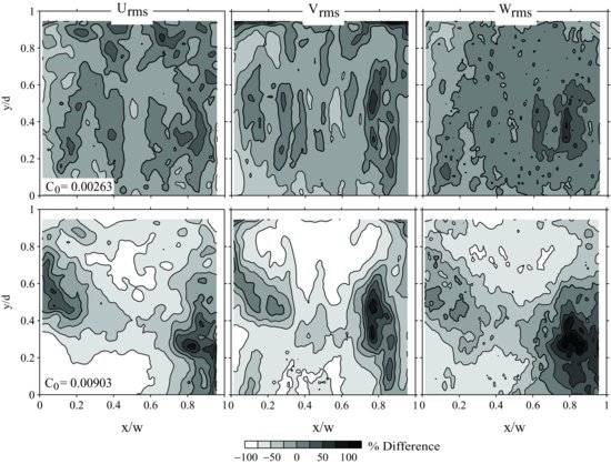
The addition of sediment has a marked effect on the fluid turbulence signal within the mixing box. Figure 20.5 shows the percentage differences between the sediment-laden and clear-water flow conditions for the root-mean-square velocity components. Modest reduction (suppression) of the turbulent velocities is observed for the supply-limited suspension for most of the flow field (up to −60%), whereas modest increases (enhancement) occur near the central nodes of the convection cells (up to +60%). Yet when the sediment concentration increases and becomes transport-limited, the turbulence reductions become much more pronounced (up to −100%), and the turbulence enhancement within the convection cells also increases in magnitude (up to +100%).
Figure 20.5 Contour plots of the percentage difference in the root-mean-square of the u, v, and w component flow velocities (left to right) within the mixing box between the clear-water conditions and the supply-limited (C0 = 0.00263, upper plots) and transport-limited (C0 = 0.00903, lower plots) conditions, shown as a function of height above the grid using a grid oscillation frequency of 2.33 Hz. The darkest contour line is 0% difference.
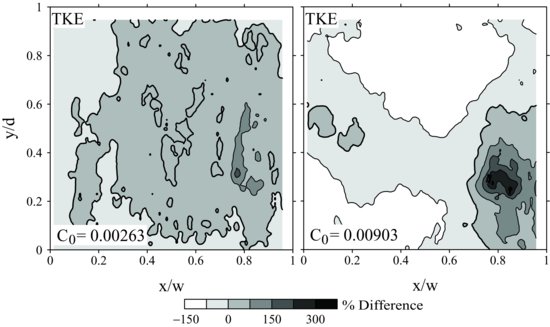
Similar trends are observed in the comparison of the clear-water and sediment-laden turbulent kinetic energy signals. For the supply-limited condition, the change in turbulent kinetic energy for the sediment-laden flow is modest, with minor amounts of suppression occurring in the central flow fields and enhanced values within the convection cells (Figure 20.6). For the transport-limited condition, the change in turbulent kinetic energy for the sediment-laden flow again is more pronounced, with greater amounts of suppression occurring in the central flow field (up to −120%) accompanied by markedly higher enhanced values within the convection cells (more than +200%). An important observation here is that both turbulence enhancement and suppression can occur within the same geophysical flow, and this phenomenon appears to depend on the relative magnitude of the turbulence and the strength of the secondary circulation.
Figure 20.6 Contour plots of the percent difference in the turbulent kinetic energy within the mixing box between the clear-water conditions and the supply-limited (C0 = 0.00263, on left) and transport-limited (C0 = 0.00903, on right) conditions, shown as a function of height above the grid using a grid oscillation frequency of 2.33 Hz. Darkest contour line is 0% difference.
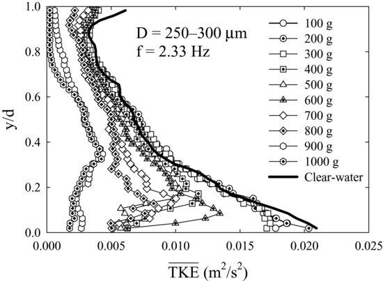
The effects of suspended sediment on the modulation of turbulence become more pronounced with increasing sediment concentration. Turbulent kinetic energy can be horizontally-averaged  for any position above the grid y/d. Figure 20.7 displays
  as a function of y/d using f = 2.33 Hz for a clear-water flow and for flows laden with 250 to 300 μm diameter sand with varying mass loadings from 100 to 1000 g. For those experiments where the input mass loading is less than 300 g (
 , the vertical profiles of
  nearly parallel those observed for the clear-water condition. Yet when the mass loadings exceed 300 g (C0>0.0039), there is a clear decrease in
  . That is, even though both turbulence suppression and turbulent enhancement occur within the same flow (see Figure 20.6), the overall (spatially averaged) fluid response at a given height above the grid is for turbulence suppression to occur. This decrease occurs throughout the water column in approximately equal amounts (as a percentage change from the clear-water value). At the highest mass loading (1000 g or C0 = 0.0130) of the 250 to 300 μm sediment, the depth-averaged
  has been reduced by nearly −80%. Although transport-limited conditions for suspended sediment occur at relatively lower mass loadings for this grain size (see Figure 20.2), turbulence within the box continues to decrease in magnitude as input concentrations increase. In related work, both Schreck and Kleis (1993) and Hussainov et al. (2000) observed a decrease in grid-generated turbulence intensity in response to an increase in sediment concentration, and these turbulent velocities decayed at faster rate with distance from the grid compared to their sediment-free conditions.
Figure 20.7 Vertical profiles above the grid of horizontally averaged turbulent kinetic energy within the mixing box as a function of input sediment loads for the 250 to 300 μm diameter sediment using a grid oscillation frequency of 2.33 Hz. Clear-water conditions also are shown.
20.4 Discussion
While the causes for the turbulence modulation remain under investigation, the magnitude and character of these signatures within this experiment are clear and unambiguous. Even with the addition of very modest concentrations of suspended sediment, significant departures of the turbulence from their clear-water values are observed. These effects are even more pronounced when the sediment-laden flow achieves transport-limited conditions, resulting in the suppression of fluid turbulence by as much as −100% within the central portion of the flow field.
The addition of suspended sediment also has a significant effect on spatially averaged flow parameters. Figure 20.8 plots the spatially averaged values (averaged in both time and space and denoted by brackets) for  ,
,  , and
, and  , velocity magnitude
  defined as
(20.4) 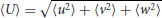
and  as a function of suspended sediment concentration C0. All flow parameters decrease as C0 increases in approximately parallel fashion, all of the trends are statistically significant, and the declines begin only when C0>0.004 (>300 g). Comparing the average values observed for C0<0.004 with those observed at the highest concentration (C0 = 0.0130), the root-mean-square values decrease by about 60%, turbulent kinetic energy decreases by about 77%, and the velocity magnitude decreases by about 56%. Finally, total spatially-averaged kinetic energy
  can be defined as
(20.5) 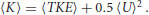
Figure 20.8 Variation in spatially averaged velocity and turbulence parameters as a function of volumetric suspended sediment concentration using a grid oscillation frequency of 2.33 Hz.
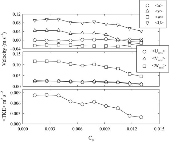
Based on the values in Figure 20.8,  is about two times larger than
  , and both parameters decrease by about 80% at the highest suspended sediment concentration (C0 = 0.0130) as compared to values measured at lower concentration (C0<0.004). This observation makes physical sense in light of the mechanics of suspended sediment. Leeder et al. (2005) showed that an upward-directed momentum flux must be required to maintain a suspended sediment load. Given that a suspended bed material load in a turbulent geophysical flow cannot take place without the transfer of momentum from the fluid to the sediment, turbulent energy should be expended in the process, which is suggested here.
Integral time and length scales for the larger eddies can be quantified as functions of suspended sediment concentration. The well known turbulent energy cascade hypothesis describes the transfer of energy from the largest scales of motion in a given flow field to smaller scales by inviscid processes, until the energy is dissipated by viscous processes at the smallest scales (Pope, 2000). The integral time scale refers to the characteristic scale of the larger eddies, and it can be calculated through autocorrelation analysis (Tennekes and Lumley, 1972; Pope, 2000). The autocorrelation coefficient  for the fluctuating cross-stream velocity component
  , for example, over time t at a given location x and y is defined as
(20.6) 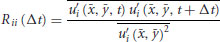
where Δt is the time lag over which the autocorrelation is calculated and the overbars signify a temporal or spatial average. The integral time scale then is determined from
(20.7) 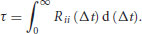
The upper limit of the integration is set by the number of time intervals, or the length of data recorded, and it is usually chosen to coincide with the first zero-crossing of the  values. Finally, using Taylor's ‘frozen turbulence’ hypothesis, the integral time scale τ can be transformed into the integral length scale λ by multiplying it by a characteristic velocity at that same location. Here, the root-mean-square velocity is used (Dohan and Sutherland, 2002; using instead the absolute value of each time-averaged velocity component had no effect on the trends reported below).
Autocorrelation analysis was applied to the sediment-laden conditions to assess turbulence modulation. Six positions in the flow field were selected for analysis (Figure 20.3) where turbulence suppression occurs (see Figures 20.5 and 20.6), and this analysis included all velocity components and all suspended sediment concentrations. Figures 20.9 and 20.10 show the variation in the integral time and length scales derived for each velocity component at each of the six locations. In general, 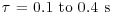 , which is very close to the oscillation period of the grid (0.43 s), and
 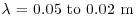 , which is very close to the bar thickness (0.01 m) and the mesh size (0.04 m) of the grid (see Dohan and Sutherland, 2002). These observations support the precept that the autocorrelation analysis quantifies the characteristic scales of the larger eddies, which should be strongly correlated to the oscillation frequency and dimensions of the grid.
Figure 20.9 Variation in the integral time scale for all three velocity components at six locations as a function of volumetric suspended sediment concentration using a grid oscillation frequency of 2.33 Hz. Refer to Figure 20.3 for point locations.
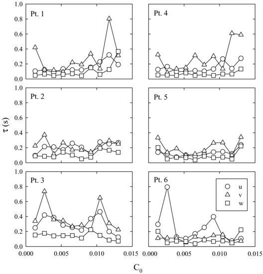
Figure 20.10 Variation in the integral length scale for all three velocity components at six locations as a function of volumetric suspended sediment concentration using a grid oscillation frequency of 2.33 Hz. Refer to Figure 20.3 for point locations.
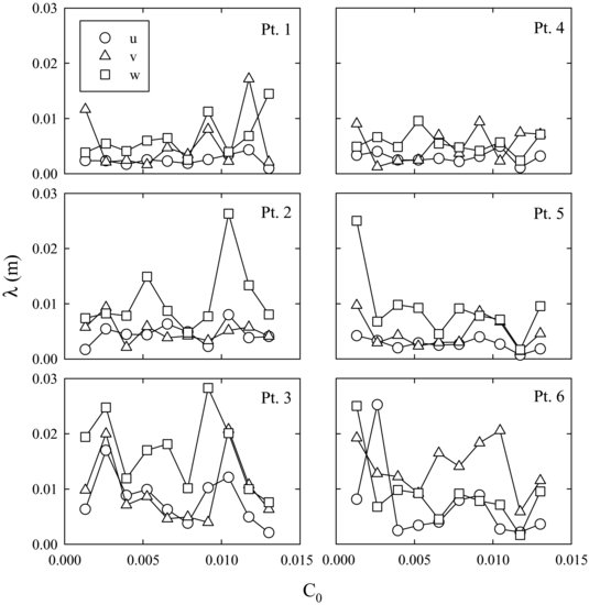
The time-mean and turbulent velocities show a systematic variation with increasing suspended sediment loads, but integral time and length scales derived from velocity time series do not. For τ, only the u and v components for Point 1 display a statistically significant (positive) trend with C0; all remaining components and positions show no statistically significant trend (Figure 20.9). For λ, no statistically significant trend with C0 is observed for any velocity component at any location examined (Figure 20.10). In addition, there is no correlation between the percentage difference in turbulent kinetic energy, as defined in Equation (20.3), and the derived turbulence time or length scales (not shown here). In sum, the decrease in turbulent kinetic energy within the mixing box due to the increase in suspended sediment concentration is not accompanied by a change in the integral time and length scales at select positions, and no correlation exists between the change in turbulent kinetic energy and these characteristic parameters.
These observations of turbulent kinetic energy and the time and length scales have important implications to the understanding of turbulence modulation in geophysical flows by suspended sediment. First, integral time τ and length scales λ for grid-generated turbulence can be related to turbulent kinetic energy TKE and the rate of dissipation of this energy  using
using
(Pope, 2000). For the experiments, turbulence production within the box is generated by the oscillation of the grid, which remains constant throughout. This oscillating grid produces turbulent kinetic energy that advects and diffuses with distance from the grid, and this energy then is dissipated at a rate given by . Given that TKE decreases with increasing C0 while both τ and λ remain unchanged, then the rate of dissipation of turbulent energy also must decrease as C0 increases using Equation (20.8). It is contended here that the reduction in TKE in the flow is due to the transfer of this energy to the sediment in suspension.
Second, any criteria used to quantify the effects of suspended sediment on turbulence based on integral time and length scales cannot be used to explain the observations reported herein. Hou (2011) used these data, as well as those derived for additional grain sizes, to critically assess the turbulence modulation criterion proposed by Gore and Crowe (1989). That is, fluid turbulence is enhanced when  and suppressed when
  . Hou (2011) demonstrated that this criterion cannot be used for data collected here, since no correlation exists between
  and the percentage difference in turbulent kinetic energy. This same criterion recently has been criticized by Tanaka and Eaton (2008), and its range of application was further qualified by Lucci et al. (2011).
Finally, density stratification can occur in zero mean-shear flows due to the presence of suspended sediment and this could affect turbulence. Noh and Fernando (1991) suggested that the existence of a horizontal front (lutocline), across which the diffusion of particles and turbulent energy are inhibited, can be identified by the shape of the vertical concentration profile. That is, when  decreases to zero monotonically, no front exists. Whereas when
  first increases with y, then decreases rapidly to zero, a front exists, and the location inflection point (
 ) can be used as the depth of the suspension layer. The suspended sediment profiles for the transport-limited condition shown in Figure 20.2b could support this stratification thesis, but a definitive analysis of this effect requires a more complete database of suspended sediment concentration. It is important to note, however, that the vertical profile of
  corresponding to the transport-limited suspended sediment profile shown in Figure 20.2b, (the 700 g profile in Figure 20.7) displays no marked deviations at greater heights away from the grid indicative of density stratification. The consideration of additional physical mechanisms for turbulence modulation could help explain some of the apparent inconsistencies and ambiguities observed in sediment-laden open channels as well as other geophysical flows.
20.5 Conclusions
The effects of a suspended sediment load on fluid turbulence in open channel flows have long been discussed. It was contended here that the use of particle image velocimetry and a standard mixing box can improve upon this previous work by employing two important experimental considerations: the creation of hydrodyamically equivalent flows, and the unambiguous discrimination of the fluid phase within sediment-laden flow. The objectives of the current paper were to quantify the time-mean and turbulent flow field within a mixing box using clear-water conditions, and to quantify the variations in these turbulent parameters in the presence of quartz-density suspended sediment using a range of input concentrations.
Turbulent flow within a mixing box was quantified using PIV and fluorescent tracer particles for the fluid phase. Flow was characterized by two depth-scale convection cells whose central portion was dominated by highly turbulent, upward-directed secondary flow velocities. Upon the introduction of quartz-density sand to the box, both turbulence enhancement and suppression were observed, but the overall effect was to decrease turbulence when compared to the equivalent clear-water flow. This result makes physical sense because energy is expended to lift the sediment mass from the bottom. Turbulence and total turbulent kinetic energy decreased markedly as suspended sediment concentration increased, and these reductions appear to coincide with decreased rates of turbulence dissipation. While the actual mechanisms for turbulence modulation remain to be determined, these results showed that under ideal experimental conditions the effects of a suspended load on fluid turbulence in a zero mean-shear flow were clear and unambiguous: the presence of suspended sediment decreased fluid turbulence. These reductions were not correlated to changes in the time and length scales of turbulence, hence any turbulence modulation criteria based on these parameters also cannot be applied. Finally, these results should be applicable to wide-range of sediment-laden geophysical flows.
20.6 Acknowledgement
This work has been financially supported by NSF-EAR 0640617 and NSF-EAR 0549607. This paper benefitted from the helpful reviews of Jeremy Venditti, Scott Wright, and an anonymous referee.
References
Balachandar, S. and Eaton, J.K. (2010) Turbulent dispersed multiphase flow. Annual Review of Fluid Mechanics 42, 111–133.
Bennett, S.J., Bridge, J.S. and Best, J.L. (1998) Fluid and sediment dynamics of upper-stage plane beds. Journal of Geophysical Research 103, 1239–1274.
Best, J.L., Bennett, S.J., Bridge, J.S. and Leeder, M.R. (1997) Turbulence modulation and particle velocities over flat sand beds at low transport rates. Journal of Hydraulic Engineering 123, 1118–1129.
Bridge, J.S. and Bennett, S.J. (1992) A model for the entrainment and transport of sediment grains of mixed sizes, shapes and densities. Water Resources Research 28, 337–363.
Dohan, K. and Sutherland, B.R. (2002) Turbulence time scales in mixing box experiments. Experiments in Fluids 33, 709–719.
Elghobashi, S. (1994) On predicting particle-laden turbulent flows. Applied Scientific Research 52, 309–329.
Gore, R.A. and Crowe, C.T. (1989) Effect of particle size on modulating turbulent intensity. International Journal of Multiphase Flow 15, 279–285.
Gore, R.A. and Crowe, C.T. (1991) Modulation of turbulence by a dispersed phase. Journal of Fluids Engineering 113, 304–307.
Hetsroni, G. (1989) Particles-turbulence interaction. International Journal of Multiphase Flow 5, 735–746.
Hopfinger, J. and Toly, J.-A. (1976) Spatially decaying turbulence and its relation to mixing across density interfaces. Journal of Fluid Mechanics 78, 155–175.
Hou, Y. (2011) Turbulence Modulation by Suspended Sediment Within a Mixing Box. M.S. thesis, University at Buffalo, Buffalo, NY.
Hussainov, M. Kartushinsky, A., Rudi, Ü. et al. (2000) Experimental investigation of turbulence modulation by solid particles in a grid-generated vertical flow. International Journal of Heat and Fluid Flow 21, 365–373.
Leeder, M.R., Gray, T.E. and Alexander, J. (2005) Sediment suspension dynamics and a new criterion for the maintenance of turbulent suspensions. Sedimentology 52, 683–691.
Lucci, F., Ferrante, A. and Elghobashi, S. (2011) Is Stokes number an appropriate indicator for turbulence modulation by particles of Taylor-length-scale size? Physics of Fluids 23, 025101.
McKenna, S.P. and McGillis, W.R. (2004) Observations of flow repeatability and secondary circulation in an oscillating grid-stirred tank. Physics of Fluids 16, 3499–3502.
Michallet, H. and Mory, M. (2004) Modelling of sediment suspensions in oscillating grid turbulence. Fluid Dynamics Research 35, 87–106.
Muste, M., Yu, K., Fujita, I. and Ettema, R. (2005) Two-phase versus mixed-flow perspective on suspended sediment transport in turbulent channel flows. Water Resources Research 41, W10402, DOI: 10.1029/2004WR003595.
Noh, Y. and Fernando, H.J.S. (1991) Dispersion of suspended particles in turbulent flow. Physics of Fluids A3, 1730–1740.
Pedocchi, F., Ezequiel, J.M. and García, M.H. (2008) Inexpensive fluorescent particles for large-scale experiments using particle image velocimetry. Experiments in Fluids 45, 183–186.
Pope, S.B. (2000) Turbulent Flows, Cambridge University Press, New York.
Schreck, S. and Kleis, S.J. (1993) Modification of grid-generated turbulence by solid particles. Journal of Fluid Mechanics 249, 665–688.
Tanaka, T. and Eaton, J.K. (2008) Classification of turbulence modification by dispersed spheres using a novel dimensionless number. Physical Review Letters 101, 114502.
Tennekes, H. and Lumley, J.L. (1972) A First Course in Turbulence, MIT Press, Cambridge, MA.
Thompson, S.M. and Turner, J.S. (1975) Mixing across an interface due to turbulence generated by an oscillating grid. Journal of Fluid Mechanics 67, 349–368.