22
Turbulence Structure and Sand Transport over a Gravel Bed in a Laboratory Flume
ABSTRACT
Characterizing the turbulence generated by flow over rough beds has become increasingly important in support of efforts to predict sediment transport downstream of dams. In many cases, fine sediments are reintroduced to coarse substrates that have large volumes of pore space available for storage. The roughness and porosity of the coarse substrate are affected by the fine sediment elevation relative to the coarse substrate. Experiments at the USDA-ARS-National Sedimentation Laboratory have focused on measurements of turbulence and sand transport over and through coarse substrates. Measurements of sand transport rate, bed texture, and bed topography were collected at four different discharges for eleven elevations of sand in the gravel bed. A collapse of the transport data was accomplished by relating the sand transport rate to the bed shear stress scaled by the square root of the value of the cumulative probability distribution function of the gravel surface evaluated at the height of the mean sand bed. The increasing elevation of sand relative to the gravel layer resulted in decreased Reynolds stress and turbulence intensity. Clear differences in turbulence structure, indicated by quadrant analysis, were observed as sand filled the upper levels of pore space.
22.1 Introduction
The interaction of a coarse streambed with flow and sediment is complex, and the controlling factors, such as bed roughness, water surface slope, coherent turbulence structures, and availability of fine sediments, are difficult to measure. However, planning for reservoir flushing or dam removal requires knowledge of these interactions. The sediment bed of rivers downstream of dams often becomes armored with gravel and deficient in sand sized sediment (Hathaway, 1948; Vanoni, 1975, p. 8). Tributaries downstream of dams, reservoir flushing, dam bypassing, or dam removal can intermittently introduce large amounts of sand to armoured gravel bed channels. In each case, sediment may be reintroduced to downstream channel beds that have had fine particles removed without replacement from upstream, leaving open pore space that can affect turbulence scales as well as providing storage capacity for flushed sediments. The proportion of a gravel bed stream that is covered by sand at the time of additional sand input strongly affects the amount of sediment transported; however, the relationship between bed coverage, transport rate, and bed shear stress is poorly understood (Grams and Wilcock, 2007).
There have been a number of studies that have investigated the effect of sand on the transport of sand-gravel sediment mixtures (e.g. Iseya and Ikeda, 1987; Ferguson et al., 1989; Kleinhans, 2002; Wilcock and Kenworthy, 2002; Curran and Wilcock, 2005; Tuijnder, 2009, 2010). It has been shown that the bed material load of streams with sand gravel beds may be reasonably predicted by using an adjustment factor to predict the critical shear stress for each size fraction relative to the mean fraction and a common transport relation (Wilcock and Crowe, 2003; Almedeij et al., 2006). While these approaches yield reasonable results for transport of generally continuous mixtures of sand and gravel, the techniques tend to break down when the sand is being transported among much larger immobile gravel. Large particles that generate vortices from separated flows and varying levels of penetration of turbulent structures into permeable beds, caused by different levels of sand in the immobile substrate, are some of the factors that impede a mechanistic understanding of the relationship between turbulence and sand transport in these conditions.
Coherent structures have a profound influence on the structure of turbulence and the ability of a flow to transport sediments, making their study necessary for the advancement of fluvial hydraulics. The present study is focused on turbulence structure and sediment transport over an immobile gravel bed. Turbulence data were collected using spatially averaged point measurements collected with an acoustic Doppler velocimeter (ADV). Although particle image velocimetry (PIV) is a valuable tool for measuring fluid turbulence (see, e.g. Sambrook Smith and Nicholas, 2005; Adrian, 2007; Hardy et al., 2010), it can be difficult to use PIV in sediment-laden flows. Several previous investigators have inferred characteristics of coherent flow structures using point measurements in sediment-laden flows in both the laboratory (e.g. Nelson et al., 1995; Bennett and Best, 1996; Wren et al., 2007; Aberle et al., 2008) and in the field (e.g. Kostaschuk and Church, 1993; Buffin-Belanger et al., 2000; Lamarre and Roy, 2005). The following paragraphs will briefly describe some previous measurements of turbulence structure that were accomplished with point measurements and their contributions to the understanding of turbulence structure.
Lapointe (1993) used turbulence and optical backscatter suspended sediment measurements to link coherent structures to sand transport in a sand bed river and Venditti and Bennett (2000) used a similar approach in a laboratory flume. Nikora and Goring (2002) used ADVs to link fluctuations in suspended-sediment concentration to turbulence. Wren et al. (2007) used acoustic backscatter and a laser Doppler velocimeter in the laboratory to assess the connection between turbulent quadrants and near-instantaneous sediment concentration. Kirkbride and Ferguson (1995) measured coherent structures over rough beds, in the form of high and low-speed wedge structures. Buffin-Belanger and Roy (1998) used an array of electromagnetic current meters (ECMs) to collect detailed turbulence data around a naturally formed pebble cluster. They found that the shedding of vortices from the cluster was the primary mechanism of turbulence generation and they also documented strong events comprised of fast moving fluid directed toward the bed in the reattachment zone and away from the bed in a region of upwelling flow. Lamarre and Roy (2005) used vertical arrays of ECMs to collected velocity profiles in a reach of a gravel bed river whose bed surface was poorly sorted with a D84 around 100 mm. They were able to quantify the integral length scales and frequency and duration of turbulent flow structures, and found that the characteristics of these structures were affected in predictable ways by local bed topography. Lamarre and Roy (2005) also detected the presence of high and low speed wedges of fluid, which were attributed to flow acceleration and vortex shedding around obstacles in the flow. In contrast to the present work, it should also be noted that the studies that were briefly described in this paragraph employed simultaneous measurements from several elevations. These studies have the advantage of allowing point-to-point correlation of instantaneous velocity fluctuations.
One way to expand the usefulness of point measurements for investigating turbulence structure is to use spatial/temporal averaging techniques that are referred to as double averaging (Nikora et al., 2007a; McLean and Nikora, 2006). The development and use of double averaging involves dividing the flow field over a rough bed into horizontal layers whose flow characteristics are defined by their position relative to the rough bed (Nikora et al., 2007b) and application of statistical techniques for describing the bed roughness (Nikora et al., 1998). Several recent works have used these techniques to examine a variety of flows over rough beds (e.g. Manes et al., 2007; Aberle et al., 2008; Cooper and Tait, 2008; Mignot et al., 2009). A condition for double averaging is that the vertical distribution of bed roughness does not change or changes slowly with time (Nikora et al., 2007a). This condition makes the use of double-averaging techniques less straightforward when the distribution of bed roughness or porosity is variable in time, such as for mobile gravel or sand patches moving through the measurement section. Direct use of the procedure for analysis of data collected with fine-grained sediment moving through a coarse substrate may require monitoring the elevation of the moving bed throughout the test section, which presents some measurement difficulties. By assuming that the mean level of the mobile fraction is steady over the measurement period, area averaging in planes parallel to the bed can be appropriate when the goal is to characterize large-scale changes in flow conditions without adding bias caused by local bed topography. This approach has been called superficial double averaging (Mignot et al., 2009).
In the present work, changes in turbulence and sand transport resulting from the addition of sand to an immobile gravel bed were investigated. Flow measurements were made at four discharges for six mean sand elevations. Sand transport measurements were made for eleven different mean bed elevations. Analyses of turbulence data, quadrant analysis, an investigation of turbulence macroscales, and the development of a predictive method for sand transport are presented. The use of spatially-averaged single point measurements to study coherent turbulent structures, as described here, shows both the limits and possibilities of the approach. The interpretation of this data set expands the current understanding of sand transport in partially filled porous beds, such as those covered by mixtures of sand and gravel. Improved understanding of the mechanistic relationship between turbulence structure and sand transport in such systems is necessary for addressing problems of prediction in sediment. Related work by the authors of this manuscript can be found in Wren et al. (2011) and Kuhnle et al. (2013).
22.2 Materials and methods
22.2.1 General methodology
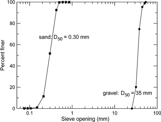
The experiments were carried out at the United States Department of Agriculture, Agricultural Research Service, National Sedimentation Laboratory in a 15 m (L) × 0.36 m (W) × 0.46 m (D) sediment and water recirculating flume with adjustable slope and a frequency-controlled motor. The sand used in the experiments ranged in size from 0.1 to 0.5 mm in diameter with a median of 0.30 mm, and (D84 D−116)1/2 = 1.35 (Figure 22.1). The gravel substrate, which was not transported in the experiments, consisted of a randomly placed layer beginning 1.2 m downstream of the head box of the channel and continuing for 13.4 m to just upstream of the tail box with mean and maximum elevations of 17.5 and 24.4 cm above the bottom of the flume channel, respectively. The gravel ranged in diameter from 27 to 52 mm with a median diameter of 35.0 mm and (D84 D−116)1/2 = 1.15 (Figure 22.1).
Figure 22.1 Grain size distributions of sand and gravel fractions.
The narrow size distribution of the gravel is not common in streams; however, the study was designed for investigating processes rather than for emulating a specific set of natural conditions. The main goal of the experiments was to study the effects of sand filling a gravel bed and so the only variables that changed were the mass of sand in the bed, the flow rate, and the flume slope, which was adjusted as necessary to maintain uniform conditions. Other recent works have also approached the study of flows over rough beds by simplifying the problem relative to natural streams. For example, Grams and Wilcock (2007) used a substrate of man-made hemispheres, and Mignot et al. (2009) used randomly placed angular gravel.
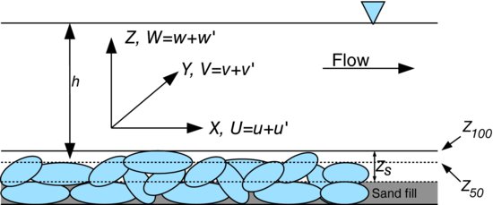
The coordinate system used in the study was as follows: X = streamwise direction and u = streamwise velocity, positive away from datum at flume entrance; Y = cross-stream direction and v = cross-stream velocity, positive away from datum at right flume wall facing downstream; and Z = vertical direction and w = vertical velocity, positive up from the datum at the flume floor (Figure 22.2).
Figure 22.2 Definition sketch for coordinate system and main variables. Zs is the distance from the maximum gravel elevation to the mean level of the sand. Z100 is the gravel elevation for which 100% of the gravel elevations are lower. Z50 is the gravel elevation for which 50% of the gravel elevations are lower.
An acoustic sensor that traversed the length of the flume along its centreline-measured water-surface slope. The average slope of all, excluding the maximum and minimum, traverses from each daily data collection session was used with the pre-run static slope to find the dynamic water surface slope. Three slope measurements were collected at the beginning, midpoint, and end of each daily flume run, for a total of nine measurements. Discharge, Q, was obtained from a calibrated Venturi meter in the return line. The cross-sectionally averaged flow velocity was calculated using  , where A is the cross-sectional area of the flowing water. Mean water depth, h, was measured during each experiment using acoustic probes to identify the water surface and bed elevations at the flume centreline. Water depth measurements were made during the slope traverses, both referenced to the datum at the flume bottom, defining the mean water depth for each traverse. Froude number, Fr, was determined from
 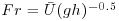 , where g is acceleration due to gravity. Wall corrected bed shear stress was determined from
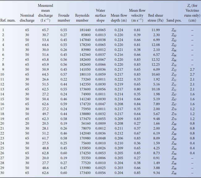
  , where ρ is fluid density. The wall correction was based on modifications of the Vanoni and Brooks (1957) method described in Vanoni (1975) with further modification by Chiew and Parker (1994), which resulted in an explicit relation for wall friction. Flow uniformity was checked for each experiment by measuring the slope of the water surface relative to the flume rails. The water surface slope deviated from the bed surface slope by an average of approximately 1 cm over the 15 meter flume length, indicating that flow conditions were approximately uniform. See Table 22.1 for a listing of bulk properties for the flume runs described here.
Table 22.1 Parameters from the experiments. Zs is the distance from Z100 to the mean sand elevation, and is only listed for runs that included turbulence data collection.
Bed surface topography was measured using close-range terrestrial digital photogrammetry similar to Hardy et al. (2009). Images were taken with a Pentax K10D digital camera with a Pentax P-DA 18–55 mm F3.5–5.6 lens with an image resolution of 3872 × 2592 pixels. ERDAS LPS® v9.3 (Leica Geosystems, 2002) was used to extract a Digital Elevation Model (DEM) of the gravel topography (Lane et al., 2000). The resulting DEMs have a horizontal resolution of 1 mm and a mean vertical root-mean-square (rms) error of approximately 1 mm.
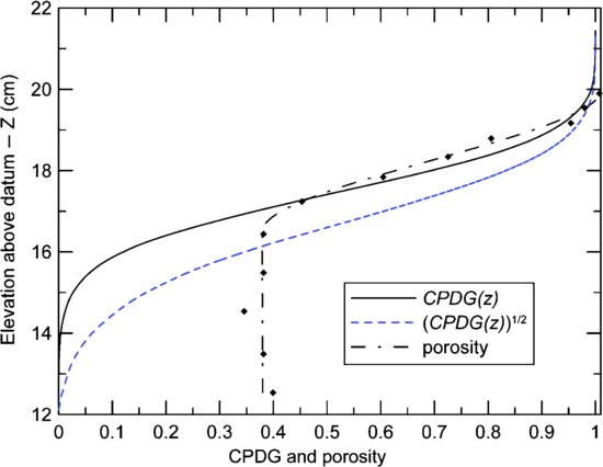
The roughness of the gravel bed was described using the Cumulative Probability Distribution of Gravel bed elevations (CPDG, Figure 22.3). The CPDG was calculated using the DEMs derived from digital photogrammetry for a 5 m long reach of the gravel bed in the channel before sand addition. This distribution represents the fraction of the solid material that is located below a particular elevation in the top layer of the bed. For instance, Z10 is the elevation for which 10% of the gravel elevations are lower. Z50, Z90, and Z100 are defined similarly. Several studies have demonstrated that the distribution of the bed elevations (Figure 22.3) is an important variable for predicting flow velocity and shear stress below the Z100 level of the bed (e.g. Manes et al., 2007; Aberle et al., 2008; Cooper and Tait, 2008; Mignot et al., 2009; Wren et al., 2011). The level of sand will be primarily referenced as the percentage of the interfacial sublayer that was filled with sand, such that sand fill to Z100 is 100%, sand fill up to Z50 is 50%, and so forth.
Figure 22.3 Cumulative probability distribution of gravel elevations (CPDG) and porosity in the bed surface. The datum is the bottom of the flume channel.
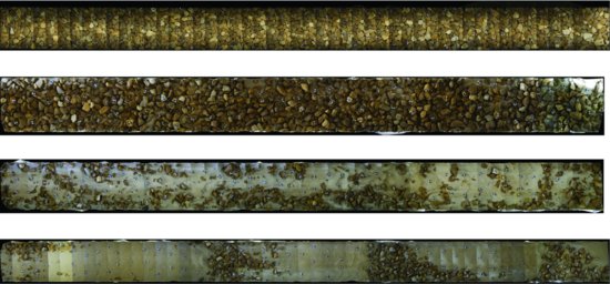
Sand was added to the channel near the downstream end and allowed to recirculate to the upstream end over several hours using a vibrating sediment feeder. The flume was run for approximately 14 hours at a discharge of 65 L s−1 to insure that the elevation of the sand had come to an equilibrium level over the length of the flume and flow was uniform. For each mean sand elevation, flow and sediment transport measurements were collected at four discharges. Figure 22.4 shows the equilibrium state of several of the sand/gravel beds. Transport data were collected for 11 different sand bed elevations from Z01 to Z98. Turbulence data were collected for six different sand elevations ranging from 0.4–2.7 cm below the maximum gravel elevation, corresponding to Z32 to Z94.
Figure 22.4 Sand addition process. The bed was allowed to reach equilibrium before transport and turbulence data were collected. Flow is from left to right.
22.2.2 Estimating sand elevation
The distance from the sand interface to the maximum gravel elevation will be designated Zs and was defined to be zero when the mean sand elevation was equal to the maximum gravel elevation. The elevation of the sand bed after the addition of 300 kg of sand was measured with a point gauge at 51 points over an 8 m length of the channel, resulting in a mean sand elevation of 5 cm below the maximum gravel elevation. The sand levels Zs < 5 cm were calculated using the porosity of the gravel and sand and the dimensions of the gravel bed in the flume. The volume of sand was based on additions of known mass with a measured porosity of approximately 0.4. The increasing porosity of the top layer of gravel, caused by the lack of an overlying gravel layer, was measured in gravel occupying an acrylic cylinder with uniform walls so that it could be used to calculate sand elevations.
22.2.3 Sediment transport
22.2.3.1 Sand transport measurements
Sediment transport was measured isokinetically in the return pipe of the flume. Total sediment transport rate was determined by catching a portion of the return line flow through a 0.053 mm sieve for low transport and by using a calibrated density cell (Dynatrol model CL-10 HYS) at 0.25 Hz for higher transport rates. Sand transport was dominated by bed load in the 20, 30, and 50 L s−1 experiments with Rouse numbers (fall velocity divided by 0.4 times shear velocity) greater than one (1.2–2.5) in all of these experiments. The 65 L s−1 experiments had more sand moving as suspended load with Rouse numbers of about 0.9, but also with significant transport of sand as bed load.
22.2.3.2 Sand transport theory
The relation between bed shear stress and sand transport rate was explored by comparing the following nondimensional quantities:
(22.1) 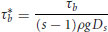
(22.2) 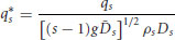
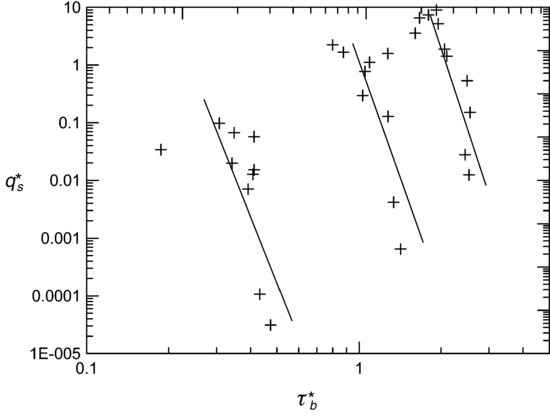
where s is ratio of the density of the sediment ( ) to the density of the water (ρ), Ds is the median diameter of the sand, and qs is the transport rate of the sand in mass per time per unit width. It is apparent (Figure 22.5) that there was a poor relation between dimensionless sand transport rate and dimensionless bed shear stress. As sand elevations in the bed increased relative to the gravel, the transport rates increased dramatically, while the bed shear stress decreased moderately.
Figure 22.5 Dimensionless sediment transport rate versus dimensionless bed shear stress for all 11 beds – the three lines illustrate negative relations between  and
and  for the experiments with flow rates of 30, 50, and 65 L s−1.
22.2.4 Turbulence measurements
22.2.4.1 Data collection
An acoustic Doppler velocimeter (ADV; Nortek Vectrino) was used to measure fluid velocity and turbulence at a rate of 200 Hz. The Vectrino used a 10 MHz beam to ensonify a region of the flow approximately 5 cm below the sensor head and collect velocities in the X, Y, and Z directions. The sampling volume was a cylinder 6 mm in diameter and 7 mm tall, resulting in a measurement volume of approximately 200 mm3. A 2 min sampling period was chosen to adequately characterize the mean and turbulent quantities while maintaining a time period feasible for collecting detailed grids of velocity data. The sampling period is comparable to that in previous laboratory and field-based turbulence studies (Lyn, 1993; Bennett and Best, 1995; Maddux et al., 2003; Buffin-Belanger and Roy, 2004; Wren et al., 2007).
The Vectrino data were collected in a single file, and an automated motion control system was used to move the instrument through a 3D grid, which had the following dimensions: X = 20 cm, Y = 10 cm, and Z = 7 cm. The single 8 h data file generated for each grid was subdivided into 2 min records and matched sequentially to the 252 locations in the sampling grid. The data were arranged into six planes parallel to the bed with elevations of (Z-Z50)/h = –0.01, 0.03, 0.08, 0.13, 0.22, and 0.31, where h = mean flow depth of approximately 21.5 cm. Each plane contained 42 points. Data were collected at Y/b = 0.22, 0.28, 0.33, 0.39, 0.44 and 0.5 relative the right flume wall, where b = 36 cm was the flume width. The most upstream sampling location was 11.8 m from the flume entrance and was defined as X = 0. Data were collected at X = 0, 3, 6, 10, 13, 16, and 20 cm. The horizontal grid dimensions were selected to be several times larger than the D50 of the gravel particles.
The effect of the sidewall on velocity profiles was checked, and it was found that, for the lowest third of the flow depth, there was no discernible effect of the sidewall at any distance greater than 5 cm from the sidewall. In a previous study performed over a sand/gravel bed in the same flume, it was found that lateral velocities were < 6% of streamwise (Horton et al., 2002). Additionally, Figure 9 of Wren et al. (2011), which is based on the same experiments as those reported here, shows the spatially-averaged bed shear stress values using the depth-slope product, Reynolds shear stress projection, and the log law for all discharges. For 65 and 50 L/s discharges, there was a 2–3 Pa spread in bed shear estimates from the three methods, which represents a range of about 25–50%. All three methods generally follow similar trends, but their magnitudes are shifted. The mean absolute difference between the depth-slope and Reynolds stress based bed shear across all discharges was 20%. The similarity between the Reynolds stress-based estimates and depth-slope estimates indicates that the effect of secondary circulation on near-bed Reynolds stresses was small.
22.2.4.2 Processing velocity data
Velocity data were separated into mean and fluctuating quantities using  where ui is a single velocity measurement and U is the mean velocity:
(22.3) 
where T = total time,  = time increment, n = total number of measurements. Vertical quantities were calculated in a similar manner. Turbulence intensities were calculated from:
(22.4) 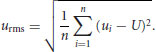
Vertical turbulence intensity was calculated in a similar manner. Reynolds stresses were calculated using
(22.5) 
where the overbar denotes time averaging.
The Vectrino data were filtered in three stages. First, all points with a correlation value below 50% for any of the velocity components were removed. Second, the data in beam coordinates were despiked with no replacement using a progressive threshold of 3.3, 3.6, and 4.3 times the standard deviation of each time series. The threshold multipliers were determined empirically through visual observation of their effects on the time series. The lower thresholds were used when the standard deviation of a dataset was greatest due to the presence of spikes, and higher thresholds were used as the standard deviation of the dataset was reduced by the removal of spikes. The increasing threshold allowed spikes to be removed while preventing the removal of good data as the standard deviation of the data was decreased by the removal of bad data points. Finally, the data were transformed into orthogonal components and despiked with no replacement using the universal threshold,  , where σ = standard deviation (Goring and Nikora, 2002). The UT is based on normal probability distribution theory and defines the maximum value expected from an independent, identically distributed, standard normal random variable. All despiking was implemented in multiple passes until the standard deviation in subsequent passes differed by less than 0.005. This series of operations prevented excessively large threshold values caused when a small number of large outliers resulted in a high value for σ, allowing spurious data to remain in the time series. Only datasets with >17 000 points (approximately 70% of the 24 000 total data points for each 2 min sampling period) were used for analyses; the mean number of points for datasets with >17 000 points was 21 490. Signal-to-noise ratios were not used in the data filtering; however, typical average values were 18 dB for lower flows and 24 dB for the highest flows. The 30 L s−1 runs had very little suspended material, so seeding particles were added. For velocity data collected in highly turbulent regions, such as near the gravel bed in the current work, despiking methods such as that described above have been shown to be an effective method for filtering ADV data (Cea et al., 2007).
22.2.4.3 Spatial averaging
Turbulence and velocity data were first processed as described above, and then spatially averaged in planes parallel to the flume bottom, where each plane covered had the following dimensions: X = 20 cm, Y = 10 cm. These dimensions are 5.7D50 in the streamwise direction and 2.9D50 laterally, which should be adequate to ensure that velocity data were collected over enough combinations of pore space and local high and low gravel elevations, especially since there was intentionally very little large-scale variation in the bed surface elevation. Spatial-averaging of time-averaged data from different locations was adopted so that global changes in flow and turbulence could be identified without interference caused by local changes in gravel elevation and unsteady effects introduced by the passage of sand through the test section. The changing local bed elevation, caused by the passage of sand patches and/or small sand bedforms, created significant challenges for defining the amount of the local pore space that was filled with sand at the time when each turbulence measurement was collected. The data were double averaged: first in time, then in space; however, the simplifying assumption that the sand bed would, on average, be at a constant level throughout the period of data collection separates the approach used here from the more comprehensive one described in, for example, Nikora et al. (2007a and 2007b). Spatial averaging over a rough bed is an accepted technique for determining global properties from local measurements (e.g. Middleton and Southard, 1984). The more recent work of Mignot et al. (2009) is another example of the use of spatial averaging across planes parallel to the bed surface for velocity measurements over gravel.
Spatial averaging was implemented over six horizontal planes with the conditions stated in the following section. For a single sampling location to be included in a horizontal plane, (1) the time series had to have npoints>17000 and (2) the local deviation of U, V, urms, wrms, and  from the spatially averaged value for that plane had to be smaller than twice the mean for that plane. Step (2) was included to ensure that datasets that were contaminated by large numbers of spikes would not be included in the spatial averages. Such datasets occurred at some elevations due to acoustic interference with the bed, which produced large numbers of spikes. For a horizontal plane to be represented in the vertical profile of spatially-averaged data,
  .
.
The principal effect of spatial averaging on the detection and measurement of coherent turbulent structures will be to mask turbulent events that do not recur regularly. Transient, low energy and local events will not be detected. The result of these limitations is that only turbulent structures that are coherent at a reach-scale and are regularly recurring will be identified using the approach employed. However, there is value in extending the interpretation of these measurements into the area of coherent structures since this can improve the mechanistic understanding of the interactions between turbulence, the rough bed, and sediment in transport.
22.2.4.4 Quadrant analysis
The structure of the Reynolds stress was examined through quadrant analysis, which was applied to each individual data set before averaging fractional contributions across horizontal planes. The quadrants are defined with the following nomenclature: quadrant 1 (Q1) events (+u′, +w′) are outward interactions, quadrant 2 (Q2) events (-u′, +w′) are bursts, quadrant 3 (Q3) events (-u′, –w′) are inward interactions and quadrant 4 (Q4) events (+u′, –w′) are sweeps (Lu and Wilmarth, 1973; Allen, 1985). For convenience, the term ‘event’ is used here, in an approach similar to that used in Lu and Wilmarth (1973), to describe a pair of simultaneous downstream/vertical velocity measurements. Bursts result from low speed fluid near the boundary moving into the relatively higher speed fluid further from the boundary. Sweeps, which result from higher speed fluid moving towards the boundary, provide an avenue for transferring momentum and energy to the near-bed region.
Turbulent events over a specified magnitude were identified by counting only those that were above a threshold value that will be referred to as the hole size, H:
(22.6) 
22.2.4.5 Turbulence scale
The downstream turbulence macroscale was determined using autocorrelation as described by Tennekes and Lumley (1978) and Hinze (1987):
(22.7) 
where T = integral time scale, and ρ(t) = autocorrelation coefficients for the fluctuating velocity time series, which were normalized by the product of n and u2rms, resulting in a peak value of ρ(t) = 1. The integral time scale, T, was approximated by summing the area under the ρ(t) curve for the first two seconds of lag time, which is equivalent to 400 values of ρ(t). Autocorrelation coefficients fluctuated slightly above and below zero beyond two seconds of lag. Hence, it was assumed that all ρ(t) for t > 2 s represented either noise or uncorrelated turbulence. The turbulence macroscale, Lx, was found by multiplying the integral time scale by the mean velocity for each time series.
22.3 Results and discussion
22.3.1 Turbulence data
Figure 22.6 shows spatially averaged Reynolds stress profiles for all discharges and elevations. For each flow rate, the Reynolds stresses are normalized by the spatially averaged mean Reynolds stress for the lowest sand elevation (i.e. τRref = τR at Zs = 2.7 cm or sand fill = 53%). The 65 L s−1 data in Figure 22.6a and the 50 L s−1 data in Figure 22.6b show a similar trend of decreasing Reynolds shear stress with increasing sand elevation, and there is no evidence of a return to the reference condition for elevations up to (Z-Z50) h−1 = 0.31. The 50 L s−1 data in Figure 22.6b show a tendency towards more similar values at high elevation, as does the 30 L s−1 data in Figure 22.6c.
Figure 22.6 The effect of sand added to a gravel bed on Reynolds stress – the legend indicates the distance of the mean elevation of the sand bed from Z100 for the gravel (the Zs elevation from Table 22.1). For each flow rate, the spatially averaged mean Reynolds (τR) stress at each elevation has been normalized by the spatially averaged mean Reynolds stress for the lowest sand elevation (τRref).
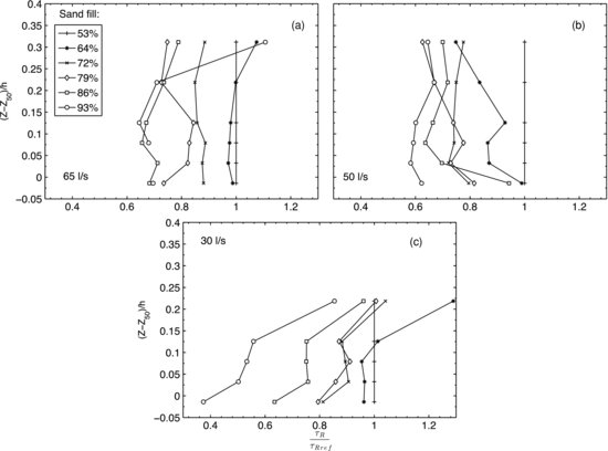
The reductions in Reynolds stress in Figure 22.6 are clearly related to the filling of pores with sand. The 30 L s−1 data in Figure 22.6c show comparable or larger reductions in Reynolds stress, relative to the reference value at 53% sand fill, compared to the 60 and 50 L s−1 data in Figures 22.6a and 22.6b. This indicates that it is very unlikely that suspended particles played a significant role in damping the turbulence. There was a large range of sediment concentrations, from negligible sediment in suspension at 30 L s−1, up to near-bed concentrations on the order of 1000 mg L−1 at 65 L s−1 for 93% sand fill.
The work of Manes et al. (2011) presents a possible mechanism for the observed reductions in Reynolds shear stress, suggesting that momentum penetration into a permeable bed increases with Reynolds number, Re = ρUh/ν, where ν = kinematic viscosity. For a given value of Re, friction factors in the Manes et al. (2011) data increased as relative roughness, h/d, where
(22.8) 
the thickness of the interface region, decreased. For impermeable beds, there was little change in the friction factor, as would be expected from the earlier results of Nikuradse (1933) for hydraulically rough flows. This dependence on h/d for permeable beds was attributed to an increase in momentum penetration into the porous bed, which also implicitly indicates an increase in effective roughness height. Here, it is indicated that the effective hydrodynamic roughness is related to the thickness of the interface region, where  is the wall porosity function and z0 is the elevation at which the total fluid stress imposed by the surface flow goes to zero (Manes et al., 2011). As the elevation of z0 decreases for a given Z100, d must increase, and more fluid momentum is transferred deeper into the pores of the rough permeable bed, increasing the force resisting the flow. Manes et al. (2011) also demonstrated an increase in the fraction of hyporheic flow as Re increased, lending more support to the hypothesis that increasing Re enhances fluid momentum penetration into a rough permeable bed. One suggested mechanism was that, as Re increased, more and more sheltered particles were subjected to flow separation, leading to growth in the total drag. The work described here is related, because, as the sand filled the bed, the elevation of z0 was gradually increased, which decreased d, limiting the depth of penetration into the permeable bed, and increasing h/d. If the hypothesis of Manes et al. (2011) is correct, another implication of the increased elevation for z0 may be a limiting effect on the growth of coherent structures caused by putting a lower elevation limit for the penetration of turbulence into the bed. It should also be noted that another contributing factor to the decrease in turbulent stresses is the reduction in energy slope that resulted from the smoother bed produced by filling of pores. In order to maintain uniform flow, the water surface slope was decreased, reducing the amount of energy available for turbulence production.
In Figure 22.7, turbulence intensity relative to the reference turbulence intensity measured with sand fill at 53% is shown. As with the Reynolds stresses, a steady decrease in turbulence intensity was observed with increasing sand elevation. There is more structure in the turbulence intensity data (Figure 22.7) than in the Reynolds stress data (Figure 22.6), with a greater relative change near the top of the coarse substrate at Z100. The relative change is less pronounced both below and above this point. Intensities may be highest near Z100 because the effect of the bed is preserved, while the sheltering/hiding/obstructing effect of roughness elements is minimized. Turbulence intensities appear to be moving back towards the reference value with increasing elevation.
Figure 22.7 The effect of sand added to a gravel bed on urms stress – the legend indicates the distance of the mean elevation of the sand bed from Z100 for the gravel. For each flow rate, the spatially averaged mean urms at each elevation has been normalized by the spatially averaged mean urms for the lowest sand elevation (urmsref).
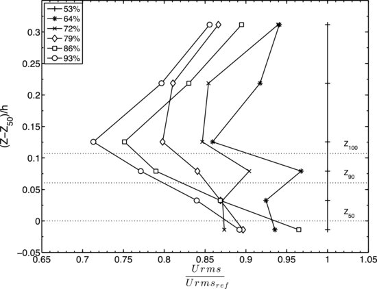
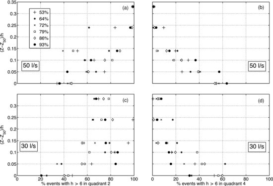
Figure 22.8 summarizes the results of spatially-averaged quadrant analysis for the 50 (Figure 22.8a & b) and 30 (Figure 22.8c & d) L/s discharges. Only data with h > 6 are shown for Q2 and Q4, based on the finding in Wren et al. (2011) that the effect of changing sand height was only clearly expressed at higher hole sizes and in Q2 and Q4. This indicates either that weaker or smaller scale structures were not affected, or that spatial averaging obscured changes to weaker turbulent structures so that only effects on stronger motions were detectable. One physical interpretation of this, when considered in light of the reductions in Reynolds stress shown in Figure 22.6, is that the Reynolds stresses were driven primarily by larger scaled higher energy structures. In Figure 22.8, for both discharges, the effect of changing the sand height was only detectable up to (Z-Z50)/h = 0.31, indicating that the influence of the bed on the turbulent structure was localized. For most of the elevations, there is not a clear progression from lower to higher sand elevations, except for the 50 L s−1 discharge at (Z-Z50)/h = 0.03 (Figure 22.8a), where it can be seen that there was a shift to a lower percentage of events in Q2 as the bed was filled. This shift was accompanied by an increase in Q4 events (Figure 22.8b) for greater sand elevations. While the shift was not clearly expressed for the smallest changes in sand elevation, it is present for the larger ones. The 30 L s−1 discharge may have been too weak to supply the energy needed to produce wakes around the gravel particles that would support strong enough turbulent structures to be detected by the methods used here. The more energetic 50 L s−1 discharge still could only produce detectable structures near the bed. In the lowest elevation, measurement difficulties and probable disruption of organized motion prevented the observations. It appears that the bursting process (Q2) was impeded by the addition of sand to the gravel matrix. Since there was also a large increase in sand transport as the elevation of sand increased, the concomitant shift to Q4 may indicate that the primary structure for entraining sediments was sweep events.
Figure 22.8 Quadrant analysis for a. Q2 at 50 L/s, b. Q4 at 50 L/s, c. Q2 at 30 L/s, and d. Q4 at 30 L/s. Each plot shows the % of events that met the h > 6 criterion and were in the stated quadrant.
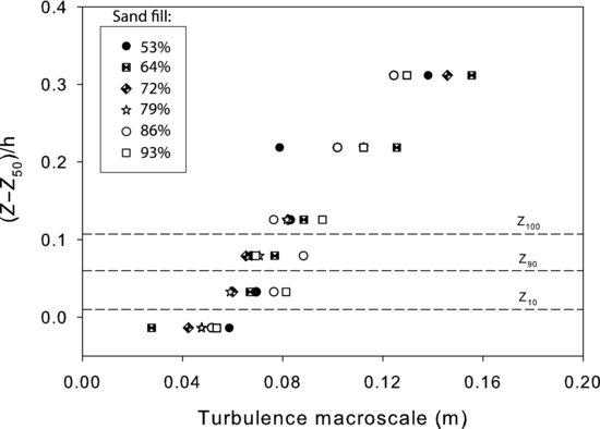
For all sand elevations, the turbulence macroscale increased with elevation, as should be expected (Figure 22.9). There is not a consistent pattern of turbulence scale with sand roughness, but there are patterns at some elevations. For (Z–Z50)/h = 0.03 – 0.12, the highest sand elevations tend to show the largest scale, while it was generally smaller for (Z–Z50)/h > 0.12. This finding is contrary to the hypothesis that limiting turbulence penetration also limits the scale of coherent structures and lends some support to the hypothesis of Nezu and Nakagawa (1993) that roughness tends to break up turbulent eddies, resulting in smaller length scales. The reduction in scale as a mechanism for decreased Reynolds stresses still seems like a more plausible explanation, especially with the significant spread in the data for each depth and fill percentage in Figure 22.9. It is likely that the relatively small changes in roughness relative to flow depth were not sufficient to affect the macroscale of turbulence strongly enough to be detected using the spatially-averaged single-point measurements described here.
Figure 22.9 Turbulence macroscales for 50 L/s.
The effect on the turbulence microscale, such as that defined by Taylor, may have been more significant. The Taylor microscale can be estimated as follows (Nezu and Nakagawa, 1993):
(22.9) 
where λ = the Taylor microscale and RL = Reynolds number in the following form:
(22.10) 
For the 50 L/s discharge, RL ≈ 13 000 and  , resulting in λ ≈ 2–4 mm, which is far smaller than the sampling volume of the acoustic Doppler probe. The sampling rate necessary to capture the Taylor microscale near the bed for this flow would be on the order of 600 Hz. The smaller turbulence scales are far too brief and small to measure with the technology used in this work; therefore, some of the effects of the changing roughness cannot be evaluated here.
22.3.2 Sediment transport relation for sand
The decreases in Reynolds stress described above were accompanied by increased sand transport. In a typical sand bed, this pairing would be paradoxical, but the increased availability of sand due to the decrease in sheltering/hiding by roughness elements makes this scenario reasonably intuitive. The near and within-bed reduction in Reynolds stresses suggest that the shear stress available for transporting sand was reduced for sand elevations below the top of the gravel. Hence, a method for reflecting the combined effect of reduced shear stress penetration and probable reductions in the scale of turbulence was needed for a predictive formulation that could link the observed changes in Reynolds stress and sand transport.
The value of the CPDG at the mean sand elevation was used as the scaling factor for the shear stress. In general, the transport of the sand in this system may be expected to have the following functional relationship:
(22.11) 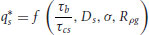
where  is the reference shear stress of the sand of size Ds which was calculated using the relation of Miller et al. (1977), σ is the standard deviation of the sediment size, and Rpg is the particle Reynolds number. If the assumption is made that the flow is in the fully rough turbulent stage when sediment is in transport, Rpg may be dropped and for moderately well sorted sand size distributions, σ may be assumed to be of secondary importance and is also dropped from consideration. This leaves a transport relation of the form
(22.12) 
in which the median size of the sand (Ds) is included in  and
and  . It is apparent from Figure 22.5 that there was not a unique relation between sand transport rate and total bed shear stress without introducing more information. To define a sand transport relation in this system, a method was needed to determine the net shear stress that was acting on the sand below the top of the gravel.
The CPDG of the surface elevation was used to scale the bed shear stress. The CPDG has several attributes that make it a good choice for this purpose. The CPDG ranges from zero at the lowest elevation of the gravel surface to a value of one at the top of the highest grain on the surface of the bed. The CPDG statistically describes the roughness of the gravel bed. When the CPDG is evaluated at the mean elevation of the sand (zs) in the gravel bed, it represents the fractional surface exposure of the sand:
(22.13) 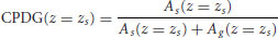
where As and Ag are the area of sand and area of gravel, respectively, at the mean elevation of the sand.
The data shown in Figure 22.5 were recast into the form of
(22.14) 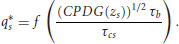
With the use of the effective shear stress, the correlation between the data is markedly improved (Figure 22.10) and is well predicted by
(22.15) 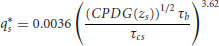
with a coefficient of determination, R2, equal to 0.92. The dashed line in Figure 22.3 shows the shape of the CPDG after raising it to the one-half power.
Figure 22.10 Dimensionless transport rate versus effective shear stress.
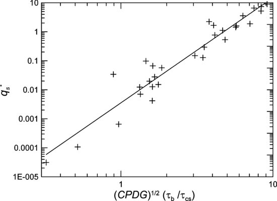
The main finding, that the shear stress affecting the sand in the gravel bed decreases with depth below the top of the gravel and may be predicted as a function of the CPDG, appears reasonable and is based on the physical distribution of the material in the top layer of the sediment bed. The scaling of the shear stress can be interpreted as limiting the shear stress that impinges on the sand layer and also takes into account changes in turbulence scale caused by the changing sand level. The collapse of the sand transport data with effective shear stress (Figure 22.10) is not perfect. In addition to the reduced or effective shear stress acting on the sand, it is likely the critical shear stress for entrainment of the sand within the gravel is significantly different than that predicted by the Miller et al. (1977) relation. It can be hypothesized that the critical shear stress for entrainment will increase for sand particles further down from the top of the gravel layer; the critical shear stress for the sand may then transition into a Shields-like relation as the sand level approaches the top of the gravel. If this functional relationship were known, it would likely allow for better collapse of the transport relationship. Additional experiments will be needed to confirm the hypothesis and quantify the relationship between sand depth and critical shear stress.
22.4 Conclusions
Turbulence and sand transport were measured over an immobile coarse gravel bed into which sand was added incrementally. The subsequent filling of the void spaces in the uppermost layer of gravel resulted in incremental reductions in Reynolds stress and turbulence intensity accompanied by increases in sand transport rate. The reductions in Reynolds stress are hypothesized to be, at least in part, the result of decreased turbulent eddy scales caused by reduced penetration of fluid momentum into the bed as the level of sand was increased. This hypothesis was extended to address the prediction of sand transport at various sand elevations relative to the gravel substrate by using a function of the value of the cumulative distribution function for gravel elevation at the mean sand elevation to scale the shear stresses acting at the sand level. This resulted in a collapse of data across a range of sand elevations and transport rates. Turbulence macroscale analysis did not produce consistent trends, leading to the conclusion that the relatively small changes in roughness relative to flow depth in our experiments may not have been large enough to produce effects that were measureable with the measurement techniques employed in this study. In the near-bed region of the more energetic flows, quadrant analysis identified a decreasing amount of strong (h > 6) Q2 events, along with an increase in strong Q4 events, as the sand elevation was increased.
References
Aberle, J., Koll, K. and Dittrich, A. (2008) Form induced stresses over rough gravel-beds. Acta Geophysica 56, 584–600.
Adrian, R.J. (2007) Hairpin vortex organization in wall turbulence. Physics of Fluids 19, 041601. DOI: 10.1063/1.2717527.
Allen, J.R.L. (1985) Principles of Physical Sedimentology, Chapman & Hall, New York.
Almedeij, J.H., Diplas, P. and Al-Ruwaih, F. (2006) Approach to separate sand from gravel for bed-load transport calculations in streams with bimodal sediment. Journal of Hydraulic Engineering 132, 1176–1185.
Bennett, S.J. and Best, J.L. (1995) Mean flow and turbulence structure over fixed, two-dimensional dunes: implications for sediment transport and bedform stability, Sedimentology 42, 491–513.
Bennett, S.J. and Best, J.L. (1996) Mean flow and turbulence structure over fixed ripples and the ripple – dune transition. In Coherent Flow Structures in Open Channels (eds P.J. Ashworth, S.J. Bennett, J.L. Best and S.J. McLelland). John Wiley & Sons, Ltd, Chichester, pp. 281–304.
Buffin-Belanger, T. and Roy, A.G. (1998) Effects of a pebble cluster on the turbulent structure of a depth-limited flow in a gravel-bed river. Geomorphology 25, 249-267.
Buffin-Belanger, T., Roy, A.G. and Kikbride, A.D. (2000) On large-scale flow structures in a gravel-bed river. Geomorphology 32, 417–435.
Buffin-Belanger, T., and Roy, A.G. (2004) 1 min in the life of a river: selecting the optimal record length for the measurement of turbulence in fluvial boundary layers. Geomorphology 68, 77–94.
Cea, L., Puertas, J. and Pena, L. (2007) Velocity measurements on highly turbulent free surface flow using ADV. Experiments in Fluids 42, 333–348.
Chiew, Y. and Parker, G. (1994) Incipient motion on non-horizontal slopes, Journal of Hydraulic Research 32, 649–660.
Cooper, J.R. and Tait, S.J. (2008) The spatial organization of time-averaged streamwise velocity and its correlation with the surface topography of water-worked gravel beds. Acta Geophysica 56, 614–642.
Curran, J.C. and Wilcock, P.R. (2005) Effect of sand supply on transport rates in a gravel-bed channel. Journal of Hydraulic Engineering 131, 961–967.
Ferguson, R.I., Prestegaard, K.L. and Ashworth, P.J. (1989) Influence of sand on hydraulics and gravel transport in a braided gravel bed river. Water Resources Research 25, 633– 643.
Goring, D.G. and Nikora,V.I. (2002). Despiking acoustic Doppler velocimeter data, Journal of Hydraulic Engineering 128, 117–126.
Grams, P.E. and Wilcock, P.R. (2007) Equilibrium entrainment of fine sediment from a coarse immobile bed. Water Resources Research 43, W10420. DOI: 10.1029/2006WR005129.
Hardy, R.J., Best, J.L., Lane, S.N. and Carbonneau, P.E. (2009) Coherent flow structures in a depth-limited flow over a gravel surface: The role of near-bed turbulence and influence of Reynolds number. Journal of Geophysical Research 114, F01003. DOI: 10.1029/2007JF000970.
Hardy, R.J., Best, J.L. Lane, S.N. and Carbonneau, P.E. (2010) Coherent flow structures in a depth-limited flow over a gravel surface: The influence of surface roughness. Journal of Geophysical Research 115, F03006. DOI: 10.1029/ 2009JF001416.
Hathaway, G.A. (1948) Observations on channel changes, degradation, and scour below dams. International Association on Hydraulic Structures, Research Project 2: Appendix 16, 287–307.
Hinze, J.O. (1987) Turbulence, 2nd edn, McGraw-Hill, New York.
Horton, J.K., Bennett, S.J., Best, J.L. and Kuhnle, R.A. (2002) Flow and Bedform Dynamics of a Bimodal Sand-gravel Mixture, USDA National Sedimentation Laboratory, Research Report 32 Oxford, MS.
Hurther, D., Lemmin, U. and Terray, E.A. (2007) Turbulent transport in the outer region of rough wall open-channel flows: the contribution of large coherent shear stress structures. Journal of Fluid Mechanics 574, 465–493.
Iseya, F. and Ikeda, H. (1987) Pulsations in bedload transport rates induced by a longitudinal sediment sorting: a flume study using sand and gravel mixtures, Geografiska Annaler 69A, 15–27.
Kirkbride, A.D. and Ferguson, R. (1995) Turbulent flow structures in a gravel-bed river: Markov chain analysis of the fluctuating velocity profiles. Earth Surface Processes and Landforms 20, 721–733.
Kleinhans, M.G. (2002) Sorting out sand and gravel: sediment transport and deposition in sand-gravel bed rivers. Netherlands Geographical Studies NGS293.
Kostaschuk, R.A. and Church, M. (1993) Macroturbulence generated by dunes: Fraser River, Canada. Sedimentary Geology 85, 25–37.
Kuhnle, R.A., Wren, D.G., Langendoen, E.J. and Rigby, J.R. (2013) Sand Transport over an immobile gravel substrate. Journal of Hydraulic Engineering 139 (2).
Lamarre, H., and Roy, A.G. (2005) Reach scale variability of turbulent flow characteristics in a gravel bed river. Geomorphology 68, 95–113.
Lane, S.N., Biron, P.M., Bradbrook, K.F. et al. (1998) Three-dimensional measurements of river channel flow processes using acoustic Doppler velocimetry. Earth Surface Processes and Landforms 23, 1247–1267
Lane, S.N., James, T.D. and Crowell, M.D. (2000) Application of digital photogrammetry to complex topography for geomorphological research. Photogrammetric Record 16, 793–821.
Lapointe, M.F. (1993) Monitoring alluvial sand suspension by eddy correlation. Earth Surface Processes and Landforms 17, 253–270.
Leica Geosystems (2002) IMAGINE OrthoBASE User's Guide, Leica Geosystems, GIS and Mapping Division, Atlanta, GA.
Lu, S.S. and Willmarth, W.W. (1973) Measurements of the structure of the Reynolds stress in a turbulent boundary layer. Journal of Fluid Mechanics 60, 481–511.
Lyn, D.A. (1993) Turbulence measurements in open-channel flows over artificial bed forms. Journal of Hydraulic Engineering 119, 306–326.
Maddux, T.B., Nelson, J.M. and McLean, S.R. (2003) Turbulent flow over three-dimensional dunes: 1. Free surface and flow response. Journal of Geophysical Research 108, 6009. DOI: 10.1029/2003JF000017.
Manes, C., Pkrajac, D., Nikora, V.I. et al. (2011) Turbulent friction in flows over permeable walls. Geophysical Research Letters 38, L03402, DOI: 10.1029/2010GL045695,
Manes, C., Pokrajac, D. and McEwan, I. (2007) Double-averaged open-channel flows with small relative submergence, Journal of Hydraulic Engineering 133, 896–904.
McLean, S.R. and Nikora, V.I. (2006) Characteristics of turbulent unidirectional flow over rough beds: double-averaging perspective with particular focus on sand dunes and gravel beds. Water Resources Research 42, W10409. DOI: 10.1029/2005WR004708.
Middleton, G.V. and Southard, J.B. (1984) Mechanics of Sediment Movement, Society of Economic Paleontologists and Mineralogists. Short Course 3, Providence, Rhode Island.
Mignot, E., Barthelemy, E. and Hurther, D. (2009) Double-averaging analysis and local flow characterization of near-bed turbulence in gravel-bed channel flows. Journal of Fluid Mechanics 618, 279–303.
Miller, M.C., McCave, I.N. and Komar, P.D. (1977) Threshold of sediment motion under unidirectional currents. Sedimentology 24, 507–527.
Nelson, J.M., Shreve, R.L., McLean, S.R. and Drake T.G. (1995) Role of near-bed turbulence structure in bed load transport and bed form mechanics. Water Resources Research 31, 2071–2086.
Nezu, I. and Nakagawa, H. (1993) Turbulence in Open Channel Flows, A.A. Balkema, Rotterdam.
Nikora, V. and Goring, D. (2000) Flow turbulence over fixed and weakly mobile gravel beds. Journal of Hydraulic Engineering 126, 679–690.
Nikora, V. and Goring, D. (2002) Fluctuations of suspended sediment concentration and turbulent sediment fluxes in an open-channel flow. Journal of Hydraulic Engineering 128, 214–224.
Nikora, V., Goring, D.G. and Biggs, B.J.F. (1998) On gravel-bed roughness characterization. Water Resources Research 34, 517–527.
Nikora, V., Goring, D., McEwan, I. and Griffiths, G. (2001) Spatially averaged open-channel flow over rough beds. Journal of Hydraulic Engineering 127, 123–133.
Nikora, V., McEwan, I., McLean, S. et al. (2007a) Double-averaging concept for rough-bed open-channel and overland flows: theoretical background. Journal of Hydraulic Engineering 133, 873–883.
Nikora, V., McLean, S., Coleman, S. et al. (2007b) Double-averaging concept for rough-bed open-channel and overland flows: applications. Journal of Hydraulic Engineering 133, 884–895.
Nikuradse, J. (1933) Laws of Flow in Rough Pipes., German Association of Engineers, Düsseldorf.
Sambrook-Smith, G.H. and Nicholas, A.N. (2005) Effect on flow structure of sand deposition on a gravel bed: results from a two-dimensional flume experiment. Water Resources Research 41, W10405. DOI: 10.1029/2004WR003817.
Tennekes, H. and Lumley, J.L. (1978) A First Course in Turbulence, MIT Press, Cambridge, MA.
Tuijnder, A.P. (2010) Sand in Short Supply, Modeling of Bedforms, Roughness, and Sediment Transport in Rivers under Supply-Limited Conditions, PhD thesis, University of Twente, The Netherlands.
Tuijnder, A., Ribberink, J. and Hulscher, S. (2009) An experimental study into the geometry of supply-limited dunes. Sedimentology 56, 1713–1727.
Vanoni, V.A. (1975) Sedimentation Engineering. American Society of Civil Engineers, New York.
Vanoni, V.A. and Brooks, N.H. (1957) Laboratory Studies of the Roughness and Suspended Load of Alluvial Streams. California Institute of Technology, Pasadena, CA.
Venditti, J.G. and Bennett, S.J. (2000) Spectral analysis of turbulent flow and suspended sediment transport over fixed dunes. Journal of Geophysical Research 105, 22 035–22 047.
Wilcock, P.R. and Crowe, J.C. (2003) A surface-based transport model for sand and gravel. Journal of Hydraulic Engineering 129, 120–128.
Wilcock, P.R. and Kenworthy, S.T. (2002) A two-fraction model for the transport of sand/gravel mixtures. Water Resources Research 38, 1194. DOI: 10.1029/2001WR000684.
Wren, D.G., Kuhnle, R.A. and Wilson, C.G. (2007) Measurements of the relationship between turbulence and sediment in suspension over mobile sand dunes in a laboratory flume. Journal of Geophysical Research 112, F03009. DOI: 10.1029/2006JF000683.
Wren, D.G., Langendoen, E.J. and Kuhnle, R.A. (2011) Effects of sand addition on turbulent flow over an immobile gravel bed. Journal of Geophysical Research 113, F01018. DOI: 10.1029/2010JF001859, 2011.