24
Interfacial Waves as Coherent Flow Structures associated with Continuous Turbidity Currents: Lillooet Lake, Canada
ABSTRACT
This study examines the role of interfacial instability in generating coherent flow structures in continuous turbidity currents in Lillooet Lake, British Columbia. Velocity and suspended sediment profiles exhibit strong vertical gradients and decrease in magnitude with height above the bed. Coarser sediment particles are concentrated below the velocity maximum while finer particles are evenly distributed within the flow. Acoustic flow visualization and local wavelet spectra show that turbidity currents display several scales of coherent flow structures, ranging from low frequency structures with a periodicity of around 3 min, to higher frequency features with periodicities of 60 s and ∼4–32 s. Values of the scale ratio of the shear layer thickness to the stratified layer thickness, and the bulk Richardson number, suggest that Kelvin–Helmholtz instability can occur during underflows with low sediment concentration and weak stratification, whilst Holmboe instabilities are more likely during underflows with higher sediment concentration and stronger stratification. Holmboe waves are an important mechanism of mixing in strongly stratified flows where turbulence is suppressed.
24.1 Introduction
Density or gravity currents are horizontal flows driven by gravity and a density difference between fluids, so that a fluid may flow over, through, or under a second fluid of a different density. Density differences between fluids may arise due to differences in temperature, chemical composition, salinity, and suspended sediment. In subaqueous environments, particulate density currents, or turbidity currents, are sediment-laden underflows that occur in less dense bodies of water, and flow downward along the bed until their load is deposited and neutral buoyancy is reached (Dufek and Bergantz, 2007). Turbidity currents commonly occur at river mouths (e.g. Best et al., 2005), as rivers laden with sediment plunge beneath the less dense receiving water body, creating a distinct ‘plunge line’. Turbidity currents are initiated by one or more processes such as landslides, debris flows, mine-tailings disposal, seismic-induced subaqueous slumps, and increased river discharge (Normark and Piper, 1991). Currents that are driven by prolonged river flow and a constant supply of suspended sediment are often referred to as ‘continuous’ turbidity currents and can persist for weeks to several months within a year (e.g. Mulder et al., 2003; Crookshanks and Gilbert, 2008).
Continuous turbidity currents are common in Lillooet Lake (Figure 24.1), a glacier-fed lake in British Columbia, throughout the glacial melt season and have been observed by Gilbert (1975), Desloges and Gilbert (1994), Best et al. (2005) and Gilbert et al. (2006). The large volume of meltwater and constant supply of glacially derived sediment delivered by Lillooet River generates strong and persistent turbidity currents in Lillooet Lake, providing a unique opportunity to obtain direct measurements of naturally-occurring continuous turbidity currents.
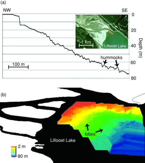
Figure 24.1 Delta front morphology. (a): Echosounder profile on 13 August 2008. The inset aerial photograph of Lillooet Delta was taken in April 2009. The red rectangle indicates the survey area for the contour map in (b). The white line within the red rectangle is the survey line for the echosounding profile and the yellow star denotes the location of the anchor station on August 13 2008. (b) Contour map based on echosounder profiles on 13 and 14 August 2008.
Modern understanding of turbidity currents relies largely on laboratory experiments (e.g. Kuenen, 1951; Garcia, 1993; Toniolo and Cantelli, 2007; Fedele and Garcia, 2008) and numerical models (e.g. Parker et al., 1987; Felix, 2002; Dufek and Bergantz, 2007; Sequeiros et al., 2009), principally due to the inherent difficulties of conducting large-scale experiments in the field that are both labour and equipment intensive. While the laboratory and numerical models cited above have provided many valuable insights into the mechanics of turbidity currents, they generally involve substantial simplification of the natural environment. Thus, quantitative field experiments are vital to validate and accurately parameterize laboratory and numerical research. Advances in field instrumentation have allowed for accurate in situ measurements, including simultaneous point measurements of suspended sediment concentration and three-dimensional velocity at varying levels in the current (e.g. Best et al., 2005).
Best et al. (2005) provided the first measurements of whole field dynamics of continuous turbidity currents in Lillooet Lake. Their study revealed the presence of velocity pulsing, or coherent flow structures (CFS), within the turbidity currents, although a steady fluvial input was present. There are at least three candidate mechanisms for these CFSs. Firstly, Best et al. (2005) suggest that the pulses may be due to shifting positions of the plunge line at the river mouth. The plunge line is characterized by distinct lobes that advance about 200 m into the lake before switching laterally. Measurements of the surface position of this surging showed a periodicity of approximately 4 min, similar to the periodicity of CFS measured in the turbidity current using an acoustic Doppler current profiler (aDcp). Dai (2008) expanded on this interpretation by proposing that the CFS may be explained as a turbulent Rayleigh–Taylor instability which, together with the momentum of the flow as it enters the lake, produces a shift in the position of the lobes along the plunge line and hence pulsing underflows.
Secondly, pulsing and related CFSs may result from convective sinking from the plunge-line lobes that extend into the lake. Parsons et al. (2001) conducted a series of laboratory experiments involving the discharge of a warm, fresh, particle-laden fluid over a relatively dense, cool brine. The surface plumes generated in the experiments were subject to a convective instability driven by heat diffusing out of the warm, fresh, sediment-laden plume and particle settling within it. Convection took the form of sediment-laden fingers that descended from the base of the surface plume and sank to the bed, generating a hyperpycnal turbidity current. The amalgamation of the sediment fingers at the bed would result in an apparent pulsing in the turbidity current. However, no evidence for this form of convection and sediment transport was observed in the present study.
The third mechanism of CFS generation, which is the focus of the present study, is interfacial wave generation at the upper interface of the turbidity current. If the shear across the interface is strong enough to overcome the stabilizing effect of the stratification, instability leads to the development of large-amplitude, wave-like structures such as Kelvin–Helmholtz (K–H) and Holmboe instabilities (Smyth and Winters, 2003; Smyth et al., 2007; Figure 24.2). Kelvin–Helmholtz instability has been investigated in more detail (see Smyth and Winters, 2003 and references therein), but conditions for Holmboe instability are common in subaqueous environments, including estuaries (Tedford et al., 2009) and river outflows (Yoshida et al., 1998). The K–H instability consists of a stationary train of billows focused at the central plane whilst the Holmboe instability is composed of a pair of oppositely propagating wave trains, focused above and below the central plane, that interfere to form a standing wavelike structure (Smyth and Winters, 2003). Holmboe and K–H instabilities can be distinguished on the basis of R, the ratio of length scales over which velocity and density change, and the bulk Richardson number, Ri (Smyth and Winters, 2003; Smyth et al., 2007) (Figure 24.2):


where hu is the thickness of the shear layer as determined from the velocity profile,  is the thickness of the stratified layer as determined from the density profile,
  is the difference in density between the fluids, g is acceleration due to gravity,
  is the mean density of the density profile, and
  is the difference in velocity between the fluids. Density (kg m−3) is a function of sediment concentration, C (g L−1), sediment grain density,
  (assumed = 2650 kg m−3), and the density of pure water,
  (kg m−3) at a temperature T (°C) (Chikita, 2007):
(24.3) 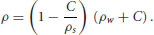
Figure 24.2 Typical velocity and density profiles (modified from Smyth and Winters, 2003, and Smyth et al., 2003), resulting from Kelvin–Helmholtz (K–H) and Holmboe (H) instabilities: u is velocity, ρ is density, hu is the thickness of the stratified layer, hρ is the thickness of the shear layer. The inset (reprinted from Tedford et al., 2009. Copyright © 2009 American Geophysical Union, with permission from John Wiley & Sons) is a schematic of a Kelvin–Helmholtz instability and a one-sided Holmboe wave.
Smyth et al. (2007) found K–H instabilities to be characterized by Ri < 0.25 and R<2 and Holmboe instabilities by Ri > 0.25 and R>2. Holmboe instabilities are thus associated with stronger density gradients compared to K–H instabilities (Figure 24.2). Importantly, mixing increases with increasing density difference in Holmboe waves, despite the fact that the transition to turbulence is delayed or prevented entirely by the stratification (Smyth et al., 2007). In addition, mixing rates in Holmboe waves are comparable to those of K–H instabilities (Smyth et al., 2003).
The purpose of the present paper is to examine mean flow and time series to determine if interfacial wave generation is a possible cause for pulsing in turbidity currents in Lillooet Lake, focusing on data collected on 13 August 2008.
24.2 Methods
24.2.1 Field measurements
A Sequoia Scientific Inc. LISST-100C laser in situ scattering transmissometer was used to provide in situ point measurements of water temperature and suspended sediment concentration (SSC) and particle size distribution at a rate of 1 Hz. The LISST uses the principle of laser diffraction to resolve particle size distribution and volumetric concentration of suspended sediment in 32 bins spaced logarithmically between 2.5 and 500 μm. A Nortek Vector acoustic Doppler velocimeter (ADV) was used to measure three-dimensional velocity at a single point, at a frequency of 1 Hz with accuracies of ± 1 mm s−1, and a sampling volume of ∼1 cm3 located 50 mm below the tip of the transmitter. An Eagle Seacharter 502 (200/500 kHz) boat-mounted single beam digital echosounder (DES) provided depth and acoustic visualization of the flow. A 500 kHz SonTek acoustic Doppler current profiler (aDcp) was deployed from the launch to provide echo-intensity measurements at a rate of 0.2 Hz. Due to instrument malfunction, the aDcp velocity sensor was inoperable during the field surveys, and so only echo-intensity was available from the aDcp. Spatial positions were determined with a Thales mobile mapper CE, which provides real-time, submeter positioning accuracy through WAAS or external differential corrections (Thales Navigation Inc., 2005). In this study, WAAS was frequently unavailable so precision was usually limited to around 5 m.
Field measurements were collected from both a moving and moored launch. At the at-a-point moorings, the ADV and LISST were deployed to provide velocity and SSC measurements and time series at several levels in the water column, whilst the aDcp was used to collect continuous profiles of echo intensity. The aDcp and DES were positioned about 2 m away from the LISST-ADV. A series of aDcp and DES transects were run along and across the delta from the moving launch, in order to examine spatial variations in bed morphology and backscatter, and to determine appropriate mooring locations. The GPS was linked to the aDcp to provide boat position and velocity corrections when conducting the surveys. The mooring sites were chosen on the basis of preliminary aDcp and DES surveys used to detect the location of the strongest underflows.
The ADV was clamped to a fixed structure attached to a rectangular frame that encased the LISST-100, and both were deployed together using a cable and boat-mounted winch. The positions of the LISST-100 and ADV were fixed so that the instruments sampled the flow at the same point in the water column. The LISST-100 and ADV were first lowered to the bed and suspended sediment and velocity data were acquired 0.1 m above the bed for 20 minutes at a frequency of 1 Hz. The instruments were then raised at 2 m intervals above the bed and the procedure repeated. Data collection was started simultaneously for the LISST, ADV and aDcp. The drift of the boat was kept at a minimum (±6 m) due to the deployment of two anchors, one at the bow of the boat and the other at the stern.
Bed-sediment samples were collected on 13 August at the mooring station to determine the particle size distribution of bed material. Additionally, suspended sediment samples within Lillooet River were taken upstream of the mooring positions to determine SSC and grain-size in the river. These sediment samples were analysed using the LISST-Portable manufactured by Sequoia Scientific Inc., which uses the same operating principles as the LISST-100.
24.2.2 Data reduction and analysis
Prior to analysis of the velocity and SSC time series, the data were screened for data quality. The velocity data from the ADV were filtered using a signal-to-noise ratio threshold value of 40, as recommended by the manufacturer. The SSC data from the LISST were screened for quality by removing all data points greater than five standard deviations from the mean of the total LISST concentration calculated over all 32 bins; this eliminated extreme outliers that sometimes occurred in the larger grain size bins due to detection of coarser material beyond the sampling range of the instrument.
The time series of velocity and SSC consist of nonstationary data that vary intermittently over time, and therefore wavelet analysis was used to determine any periodicity in the data. Wavelet analysis uses functions called wavelets that are localized in time (Farge, 1992) to show the distribution of variance at different frequencies (or scales), thus decomposing the time series into time-frequency-space to reveal localized intermittent periodicities (Torrence and Compo, 1998; Grinsted et al., 2004). The Morlet wavelet was chosen for the present analysis because it is nonorthogonal and complex. Nonorthogonal wavelets are best suited for time series analysis when continuous variations in wavelet power are expected, and a complex wavelet function returns information on both amplitude and phase and is more useful for capturing oscillatory behaviour (Torrence and Compo, 1998).
24.3 Results and discussion
There are two main distributary channels on the subaerial Lillooet delta plain (Figure 24.1). Echosounding transects showed that underflow activity was strongest at the north-eastern distributary channel, where a buoyant plume of suspended material and floating debris spread out immediately beyond the plunge line. The flow in the plume generated a recirculation zone on the flow surface with a periodicity, based on visual observation of floating debris, of about 15 minutes.
Two surface water samples taken from the eastern distributary on the delta plain on August 13 revealed SSC of 174 and 185 mg L−1 and a median grain size as 11.5 and 12.5 μm respectively. These samples were composed predominantly of fine silt-clay (< 63 μm; 87–88%). Coarser sediment is usually transported in the lower regions of the water column due to its higher settling velocities, and thus the fine fraction may have been overestimated in the surface samples and not truly representative of the average sediment composition of the river and the input to turbidity currents.
Figure 24.1 illustrates the morphology of the subaqueous delta at the mouth of the north-eastern distributary channel as derived from the bathymetric data. The delta plain, or ‘topset’, is characterized by a gently sloping surface that extends to a break in slope at a depth of approximately 5 m. The steeply sloping lakeward delta front, or ‘foreset’, has an irregular, ‘hummocky’ topography with some of the hummocks displaying a lobate form.
The turbidity currents that were measured in August 2008 were active for the one-week duration of the field study, and were probably present during the entire month as river discharges were significantly higher before and after the measurement period (Water Survey of Canada: Station 08MG005, Lillooet River near Pemberton). Although it has been suggested that inflow from Lillooet River requires a discharge greater than 300 m3 s−1 to generate underflows (Gilbert, 1975), the discharges recorded in this study (199 m3 s−1) were sufficient to generate underflows during August 2008. Continuous turbidity currents have been observed to persist for an entire month in Kluane Lake (Crookshanks and Gilbert, 2008) and several weeks in Lillooet Lake (Gilbert, 1975; Best et al., 2005). It is the substantial quantity of meltwater and glacially-derived sediment from the glaciers in the summer months that generate persistent turbidity currents in Lillooet Lake.
The SSCs of Lillooet River (∼180 mg L−1) during this study were low compared to previous measurements of 1500–2950 mg L−1 (Gilbert, 1974, 1975) during the melt season. The particle size distribution of the river samples revealed that most of the suspended sediment was finer than 63 μm, which is in agreement with the results obtained by Desloges and Gilbert (1994). The fine fraction dominates the sediment load in Lillooet River because coarser material becomes trapped in proglacial lakes (e.g. Silt Lake; Schiefer and Gilbert, 2008). Sediment from glaciers is the most consistent and primary source of suspended sediment in the river and contributes 75–83% of the clay and silt in the flow (Desloges and Gilbert, 1994).
The lake bathymetry on the north-eastern side of the delta front shows that the delta front is unchannelized, in agreement with similar observations by Best et al. (2005) and Gilbert et al. (2006). The turbidity currents generated in August 2008 can be classified as low-density hyperpycnal flows (cf. Wright et al., 1986), and such flows are unlikely to erode the bed and thereby incise channels. Indeed, such low-density turbidity currents are often laterally widespread and depositional (Wright et al., 1986). The sediment grab sample obtained from the bed on 13 August shows that fine sediment dominates the upper foreset, which agrees with sediment cores obtained from the foreset by Gilbert (1975). Thus, it is likely that sands and coarser particles transported by the Lillooet River are deposited on the upper foreset slope.
The hummocks on the foreset of the subaqueous delta have also been described by Gilbert (1975), who documented large mounds on the bed that occurred from 16 m to 120 m depth. It is possible that these mounds are relict antidune bedforms (e.g. Wynn et al., 2000, 2002; Ercilla et al., 2002; Fedele and Garcia, 2008) generated by a particularly strong turbidity current such as that during the major flood event in 2003 (Gilbert et al., 2006). The bathymetric evidence, however, indicates that the mounds are not laterally extensive and are more likely caused by mass movements and the downslope evolution of slumps. Gilbert (1975) investigated the origins of the mounds in Lillooet Lake and determined that sediment is unstable on slopes that are greater than 3.5°. Thus, the coarser sediment deposited on the upper foreset is potentially unstable and mass movement may occur to generate large slump deposits.
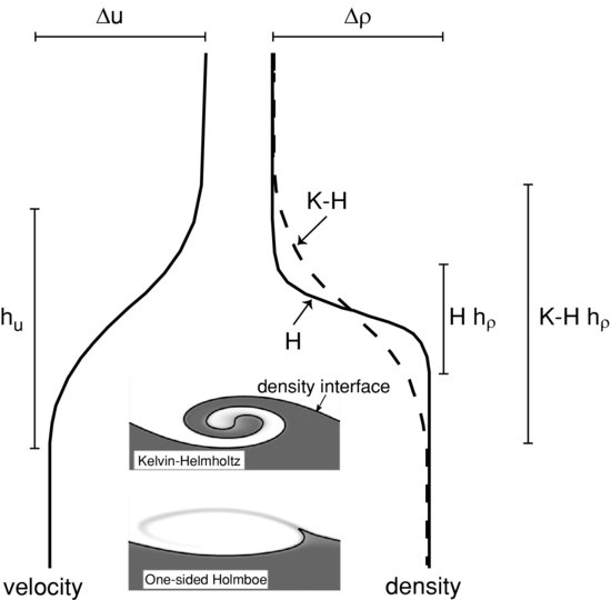
The current generated on 13 August plunged beneath the lake as an underflow at the river mouth and flowed offshore by a distance of c.300 m to a depth of about 50 m, where it became an interflow (Figure 24.3). The underflow portion of the current was characterized by large-scale CFSs with a wavelength of about 100 m.
Figure 24.3 Echosounding record offshore from the distributary mouth on 13 August 2008 (see Figure 24.1 for location). ‘Profile’ refers to the location of the ADV and LISST measurements (see Figure 24.1 for location); ‘r’ refers to ‘reflector’, an interference pattern likely caused by logs floating vertically in the lake.
Temperature, velocity and SSC profiles for 13 August are presented in Figure 24.4. Temperature decreases in a nearly linear fashion from the bed to the lake surface, with the influent river water being nearly 2.5 °C colder than the surface lake water. Velocity increased rapidly away from the bed (Figure 24.4a) to a maximum of 0.3 ms−1 at 2 m, and then decreased to 0 ms−1 at 24 m above the bed. The total and silt-clay SSC profiles are similar in shape to the velocity profile (Figure 24.4b), with maximum values at 2 m above the bed, but the sand SSC profile decreases linearly above the bed to zero at 26 m. Density, when calculated based on water temperature alone and SSC and temperature combined (Figure 24.5), is consistently highest from the bed to about 6 m and then decreases to the lake surface. The thickness of the underflow was approximately 10–12 m, as estimated by determining the distance from the bed to the inflection point of the SSC profile (e.g. Chikita, 1990; Middleton, 1993; Felix, 2002).
Figure 24.4 Mean flow structure on August 13 2008. (a): mean velocity (U), temperature (T), (b): suspended sediment concentration (SSC). hu is the thickness of the stratified layer.
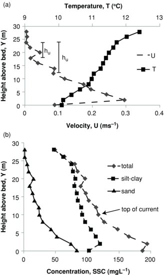
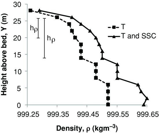
Figure 24.5 Mean water density on 13 August 2008 determined from temperature (T) and temperature and suspended sediment concentration (T and SSC); hρ is the thickness of the stratified layer.
Normark (1989) found that continuous turbidity currents occur whether lakes are thermally stratified or nearly isothermal, because temperature is thought to contribute little to the density difference between turbidity currents and the ambient lake water. However, the present study shows that, in Lillooet Lake, the density difference of river inflow and ambient lake water was dependent on both temperature and SSC, as noted earlier by Gilbert (1975). While suspended sediment contributed more to the excess density of the river inflow, the cool temperatures of the river inflow were also important in generating the excess density required for generation of hyperpycnal turbidity currents. Best et al. (2005) found that the temperature difference only generated a density excess of ∼0.018 kg m3, whereas the suspended sediment in the turbidity current generated a density excess of 0.38–0.61 kg m3. Thus, temperature contributed little to the density difference between the river inflow and ambient lake water, and it was the suspended sediment that was the driving mechanism of the turbidity currents recorded by Best et al. (2005). The temperature difference between the river inflow and ambient lake water played a more important role in generating the density difference in the present study because the SSC was much lower than the SSC of 610–980 mg L−1 measured by Best et al. (2005). The velocities of the turbidity currents in the present study were also lower than those recorded by Best et al. (2005) (Table 24.1), with the higher velocity and SSC measurements obtained by Best et al. (2005) reflecting the higher river discharges related to a flood event documented in their study.
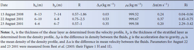
Table 24.1 Parameters used to calculate R, the ratio of length scales over which velocity and density change, and the bulk Richardson number, Ri.
The overall shape of the vertical profiles of velocity and SSC on 13 August compare reasonably well with profiles from laboratory (Choux et al., 2005; Gray et al., 2005) and field research (Chikita, 1990; Best et al., 2005). The velocity maximum was at approximately 0.2 of the total current thickness, which is in agreement with laboratory measurements (e.g. Kneller et al., 1997, 1999; Best et al., 2001; Buckee et al., 2001). The height of the velocity maximum is a function of the drag forces at the upper and lower interfaces of the turbidity current (Middleton, 1993; Kneller et al., 1997) and can be used to differentiate a lower and upper region of the underflow (Kneller et al., 1999). The turbidity currents measured in the present study clearly have a dense lower region and a less dense mixing region above the velocity maximum, at which point both the velocity and density gradients steadily decline, as observed in the laboratory study of Garcia and Parker (1993). The density profiles recorded on 13 August also compare well with the field results of Chikita (1990), where a high-density gradient in the lower part of the flow (at and below the velocity maximum) is overlain by a region of gradual decreases in density immediately above the velocity maximum in the upper mixing region.
The profiles of velocity and density on 13 August are typical of lacustrine environments with underflows. The dense, and faster moving, current in the lower regions of the water column diminishes steadily upwards in the water column as overlying less dense, and slow moving, ambient lake water is mixed and entrained into the current. The vertical distribution of SSC showed a similar upward decrease in the water column, since the high SSC in the lower part of the water column is part of the turbidity current that is much denser than the overlying ambient lake water. The SSC profile is smooth, rather than stepped, indicating the turbidity currents are weakly depositional (Peakall et al., 2000; Hosseini et al., 2006).
Suspended sediment in the turbidity current on 13 August was dominated by the silt-clay fraction. Turbidity currents typically transport fine material in suspension due to its relatively low settling velocity (Normark and Dickson, 1976; Alexander and Mulder, 2002; Pirmez and Imran 2003). It is likely that the sand component of an inflowing river settles close to the head of the lake or reservoir (Middleton, 1993; Alexander and Mulder, 2002) due to the inability of most lacustrine turbidity currents to suspend sand (Mulder and Alexander, 2001). Similar observations were made by Normark and Dickson (1976) in Lake Superior, who found that the deposition of coarse particles occurred on the upper slope, and even steep gradients were incapable of generating turbidity currents that could transport much coarse sediment in suspension. The bed sediment sample at the at-a-point mooring in the present study indicates that the sand content was less than 22%, which supports the suggestion that coarser sediment is largely deposited near the river mouth and not being transported downslope. Gilbert (1975) and Desloges and Gilbert (1994) also reported that coarser sediment (> 63 μm) accumulated near the river mouth in Lillooet Lake.
The presence of fine particles is vital in maintaining the efficiency of turbidity currents. Gladstone et al. (1998) found that smaller sizes of fine material in turbidity currents are more effective in sustaining the current, and it is this fine material that provides the current with sufficient momentum to transport some sand in suspension. The sand content in the turbidity current in Lillooet Lake mostly comprises very fine to fine sand (63–250 μm), which supports the proposition by Alexander and Mulder (2002) that fluvially generated turbidity currents are dominated by sediment finer than medium sand. In this study, the sand content in the turbidity currents steadily decreases upward away from the bed and is negligible in the uppermost part of the water column.
Figure 24.6a illustrates the time series of signal amplitude on 13 August 2008 derived from the aDcp, and Figure 24.6b shows simultaneous measurements of velocity from the aDV and SSC from the LISST. The visualization of signal amplitude shows that distinct ‘pulses’ are apparent throughout the series. The mean turbidity current flow thickness on Figure 24.6a is approximately 8–10 m, which is consistent with the estimate from the SSC profile (Figure 24.4). There are several larger flow structures that are up to 16 m thick (e.g. ∼10:05 min) and some of the larger structures (e.g. ∼10:03–10:07 min) appear to be composed of several smaller structures. There are approximately six large structures in the series shown in Figure 24.6b and approximately 15 smaller structures, with periodicities of about 3.3 minutes and 1.3 minutes respectively. The SSC time series fluctuates about a mean of ∼200 mg L−1, with a larger event at around 10:03 minutes where SSC reaches nearly 600 mg L−1. This large event may be related to a buildup of sediment at the plunge line, which is then transported downslope in a pulse. Velocity is low early in the record then increases in conjunction with the large SSC event.
Figure 24.6 Time series on 13 August 2008. (a): aDcp signal amplitude (counts) flow visualization for the water column. The broken line represents the position of the SSC and U record in (b). The SSC record (Figure 24.4) indicates that the mean top of the current is approximately 10 m from the bed; (b): aDv velocity (U) and LISST suspended sediment concentration (SSC) measured 2 m above the bed for the same time period as the aDcp. PDT refers to Pacific Daylight Time.
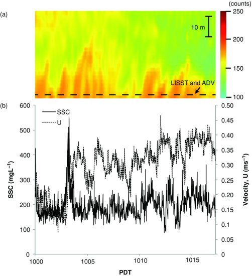
The local wavelet transforms of the velocity series (Figure 24.7) show an overall increase in variance with height above the bed. Short period (4–16 s) peaks of wavelet power occur at all heights in the turbidity current. At 6 m above the bed, longer period fluctuations of 32 s and 32–64 s are present within the time series at 400 s and 700 s respectively. At 8 m above the bed, significant structures occur in the wavelet plot at a periodicity between 16–32 s at 50 s, 400 s, 600 s, and 850 s, with a longer period structure at 400 s occurring in the 64 s band.
Figure 24.7 Local wavelet power spectrum of velocity (U) and suspended sediment concentration (SSC) on 13 August 2008 for time series (a) 2 m above the bed (see Figure 24.6b), (b) 6 m above the bed, (c) 8 m above the bed. The colour bar indicates wavelet power normalized to the time series variance, thick black contours designate the 5% significance level against red noise, and the white area indicates the cone of influence.
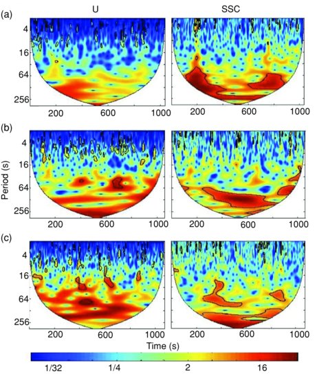
The local wavelet transforms of SSC time series (Figure 24.7) show that there is a larger range of periodicity in the SSC data, and that the variance is distributed at much longer periods compared with velocity, although short period peaks (2–8 s) are present at all heights. At 2 m above the bed, there is a large wavelet structure that occurs at varying scales between ∼32–256 s near the beginning of the series, reflecting the major SSC event in the time series at 150–250 s. Another significant peak of wavelet power occurs at 600–800 s at a periodicity of 64–128 s. At 6 m above the bed, the wavelet spectrum of SSC shows a major structure of high wavelet power at 220–810 s in the series with a periodicity of 64–200 s. Two medium-sized structures with periodicities of 64 s and 64–120 s occur at 100 s and 810 s respectively in the time series. At 8 m above the bed, a major long-period structure (∼128–256 s) occurs from 250–900 s in the series. Long period peaks (20–100 s) also occur from 250–500 s in the time series.
Table 24.1 summarizes the observations required for the calculation of the scale ratio R (Equation 24.1) and the bulk Richardson number Ri (Equation 24.2) for the 13 August 2008 data in this study, and two dates in August 2001 measured by Best et al. (2005). The instrumentation used in the present study differs from that of Best et al. (2005) but the results are comparable. It is important to note that the parameters in Table 24.1 are difficult to measure in natural turbidity currents (e.g. Crookshanks and Gilbert, 2008), resulting in uncertainty in the calculation of R and Ri. This is particularly true of the shear layer thickness, hu, and the stratified layer thickness,  . A comparison of the velocity and density profiles of the current on 13 August 2008 in Figure 24.4 and 24.5 with the idealized profiles on Figure 24.2 illustrates the subjectivity of parameterization associated with natural systems. However, the present measurements can be somewhat constrained by estimating the thickness of the density current as the distance from the bed to the inflection point of the SSC profile (e.g. Middleton, 1993; Chikita, 1990; Felix, 2002), which for the 13 August 2008 current was 10–12 m above the bed (Figure 24.4b). There is also a distinct inflection in the velocity profile at 11 m above the bed (Figure 24.4a) that is consistent with the SSC inflection, and velocity decreases to zero at 24 m above the bed, for a value of hu = 13 m. An inflection in the velocity profile is also present at 18 m above the bed (Figure 24.4a), resulting in hu = 6 m. The density profile for the 13 August 2008 current (Figure 24.5) indicates that the upper interface of the current is at the top of the upper ‘step’ of the profile at 13 m above the bed, and the top of the mixing zone is 27 m above the bed, resulting in
  . Alternatively, the upper interface of the current could be at 20 m, for a value of
  = 7 m. The August 2001 data of Best et al. (2005) are better constrained, possibly because of higher suspended sediment concentrations and a clearer distinction between the current and ambient lake water. In addition, velocity and density profiles were obtained from aDcp measurements and were simultaneous at all depths, resulting in better-defined mean profiles.
The values of R and Ri for 13 August 2008 are consistent with K–H instability (Ri < 0.25, R < 2). The 22 August 2001 values for R are indicative of both K–H and Holmboe instabilities (R < 2, R > 2), while Ri values (Ri > 0.25) imply Holmboe waves. Values of R for 23 August 2001 indicate K–H instability (R < 2) but the Ri is consistent with Holmboe instability (Ri > 0.25). If these results are accepted as reasonable, then K–H instability is likely during underflows with low sediment concentration and weak stratification and Holmboe instability during underflows with high sediment concentration and strong stratification. These results do not eliminate the processes of lobe shifting (e.g. Best et al., 2005) or convective sinking from the plunge-line lobes (e.g. Parsons et al., 2001) as causes of pulsing, although no evidence of the latter was found herein, but rather indicate interfacial wave instability as a plausible candidate.
Significant peaks in the wavelet transforms of velocity occurred at all three measured heights within the turbidity current, which suggests that the pulsations occupy most of the current and are not present just at the upper interface. A similar observation was made by Best et al. (2005) where velocity pulsing was recorded throughout the entire flow depth of the turbidity current. If interfacial waves are accepted to cause the CFSs in Lillooet Lake, then they could affect the entire thickness of the current. The wavelet transform of velocity 8 m above the bed shows that both higher and lower frequency structures are present throughout the time series. This suggests that small-scale K-H instabilities (with periodicities of 4–16 s) occur concurrently with larger-scale K–H instabilities (with periodicities of up to 64 s). Readings et al. (1972) also observed the occurrence of smaller scale K–H instabilities at the interface between larger billows, whilst Kneller and Buckee (2000) associated secondary instabilities with K–H vortex breakdown. Ellison and Turner (1959) describe this phenomenon as the ‘irregular succession of large eddies’ and this phenomenon was explained by Turner (1973) as the result of the growth and subsequent overturn or collapse (resembling spirals) of K–H instabilities, which produce patches of turbulent mixing.
24.4 Conclusions
The following conclusions can be drawn from this study of coherent flow structures associated with continuous turbidity currents in Lillooet Lake:
- Acoustic flow visualization and local wavelet spectra show that the turbidity currents display several scales of coherent flow structures. The largest structures have a periodicity of approximately 3 min, with higher frequency structures at periodicities of 60 and ∼4–32 s.
- The scale ratio of the shear layer thickness to the stratified layer thickness and the bulk Richardson number suggest that the coherent flow structures measured in this study could be caused by Kelvin–Helmholtz or Holmboe wave instabilities, although the parameters used in the calculations are difficult to constrain for natural turbidity currents.
- K–H instabilities are more likely during underflows with low sediment concentration and weak stratification, whilst Holmboe instability is more likely during underflows with high sediment concentration and strong stratification. Mixing increases with increasing density difference in Holmboe waves even when turbulence is suppressed, and mixing rates in K–H and Holmboe waves are comparable.
The results from this study, and previous field measurements of continuous turbidity currents, are limited to a few positions and fail to capture the spatial evolution of turbidity currents. It is likely that turbidity current dynamics will vary across flow, as well as downflow from the point source. A fully three-dimensional study of natural turbidity currents could be accomplished using the water column capabilities of multibeam echosounders, such as that described by Simmons et al. (2010) and Best et al. (2010). Multibeam echosounders can provide detailed visualizations of SSC and reveal the temporal evolution and growth of instabilities along mixing interfaces between two flows (Simmons et al., 2010). Such multibeam echosounders also enable centimetric resolution bathymetric mapping that would enhance the understanding of the relationship of turbidity currents and bed morphology. Advancement in the understanding of natural turbidity currents clearly relies on conducting temporally- and spatially- extensive studies that investigate the lateral variability of the passage of the underflows into the lake at multiple timescales, and relating these lateral movements to temporal variations in the turbidity current flow.
References
Alexander, J. and Mulder, T. (2002) Experimental quasi-steady density currents. Marine Geology 186, 195–210.
Bell, H.S. (1942) Density currents as agents for transporting sediments. Journal of Geology 50, 512–547.
Best, J., Kirkbride, A. and Peakall, J. (2001) Mean flow and turbulence structure of sediment-laden gravity currents: new insights using ultrasonic Doppler velocity profiling. In Particulate Gravity Currents, vol. 31 (eds W.D. McCaffrey, B.C. Kneller and J. Peakall). International Association of Sedimentologists, Ghent, pp. 159–172.
Best, J.L., Kostaschuk, R.A., Peakall, J., et al. (2005) Whole flow fleld dynamics and velocity pulsing within natural sediment-laden underflows. Geology 33, 765–768.
Best, J., Simmons, S., Parsons, D. et al. (2010) A new methodology for the quantitative visualization of coherent flow structures in alluvial channels using multibeam echo sounding (MBES). Geophysical Research Letters 37, L06405. DOI: 10.1029/2009GL041852.
Buckee, C., Kneller, B. and Peakall, J. (2001) Turbulence structure in steady, solute-driven gravity currents. In Particulate Gravity Currents, vol. 31 (eds W.D. McCaffrey, B.C. Kneller and J. Peakall). International Association of Sedimentologists, Ghent, pp. 173–187.
Chikita, K. (1990) Sedimentation by river-induced turbidity currents: field measurements and interpretation. Sedimentology 37, 891–905.
Chikita, K. (2007) Topographic effects on the thermal structure of Himalayan glacial lakes: observations and numerical simulation of wind. Journal of Asian Earth Sciences 30, 344–352.
Choux, C.M.A., Baas, J.H., McCaffrey, W.D. and Haughton, P.D.W. (2005) Comparison of spatio-temporal evolution of experimental particulate gravity flows at two different initial concentrations, based on velocity, grain size and density. Sedimentary Geology 179, 49–69.
Crookshanks, S. and Gilbert, R. (2008) Continuous, diurnally fluctuating turbidity currents in Kluane Lake, Yukon Territory. Canadian Journal of Earth Sciences 45, 1123–1138.
Dai, A. (2008) Analysis and Modeling of Plunging Flows. Unpublished PhD thesis, Department of Civil and Environmental Engineering, University of Illinois at Urbana-Champaign, IL.
Desloges, J.R. and Gilbert, R. (1994) Sediment source and hydroclimatic inferences from glacial lake sediments: the post-glacial sedimentary record of Lillooet Lake, British Columbia. Journal of Hydrology 159, 375–393.
Dufek, J. and Bergantz, G.W. (2007) Suspended load and bed-load transport of particle-laden gravity currents: the role of particle-bed interaction. Theoretical Computational Fluid Dynamics 21, 119–145.
Ellison, T.H. and Turner, J.S. (1959) Turbulent entrainment in stratified flows. Journal of Fluid Mechanics 6, 423–448.
Ercilla, G., Alonso, B., Wynn, R.B. and Baraza, J. (2002) Turbidity current sediment waves on irregular slopes: observations from the Orinoco sediment-wave field. Marine Geology 192, 171–187.
Farge, M. (1992) Wavelet transforms and their applications to turbulence. Annual Review of Fluid Mechanics 24, 395–457.
Fedele, J.J. and Garcia, M.H. (2008) Laboratory experiments on the formation of subaqueous depositional gullies by turbidity currents. Marine Geology 258, 48–59.
Felix, M. (2002) Flow structure of turbidity currents. Sedimentology 49, 397–419.
Garcia, M.H. (1993) Hydraulic jumps in sediment-driven bottom currents. Journal of Hydraulic Engineering 119, 1094– 1117.
Garcia, M.H. and Parker, G. (1993) Experiments on the entrainment of sediment into suspension by a dense bottom current. Journal of Geophysical Research – Oceans 98, 4793–4807.
Gilbert, R. (1974) Observations of Lacustrine Sedimentation at Lillooet Lake, British Columbia. Unpublished PhD Thesis, University of British Columbia, Vancouver, Canada.
Gilbert, R. (1975) Sedimentation in Lillooet Lake. Canadian Journal of Earth Sciences 12, 1697–1711.
Gilbert, R., Crookshanks, S., Hodder, K.R. et al. (2006) The record of an extreme flood in the sediments of montane Lillooet Lake, British Columbia: implications for paleoenvironmental assessment. Journal of Paleolimnology 35, 737–745.
Gladstone, C., Phillips, J.C. and Sparks, R.S.J. (1998) Experiments on bidisperse, constant-volume gravity currents: propagation and sediment deposition. Sedimentology 45, 833–843.
Gray, T.E., Alexander, J. and Leeder, M.R. (2005) Quantifying velocity and turbulence structure in depositing sustained turbidity currents across breaks in slopes. Sedimentology 52, 467–488.
Grinsted, A., Moore, J.C. and Jevrejeva, S. (2004) Application of the cross wavelet transform and wavelet coherence to geophysical time series. Nonlinear Processes in Geophysics 11, 561–566.
Hosseini, S.A., Shamsai, B. and Ataie-Ashtiani, B. (2006) Synchronous measurements of the velocity and concentration in low-density turbidity currents using an Acoustic Doppler Velocimeter. Flow Measurement and Instrumentation 17, 59–68.
Kneller, B.C., Bennett, S.J. and McCaffrey, W.D. (1997) Velocity and turbulence structure of gravity currents and internal solitary waves: potential sediment transport and the formation of wave ripples in deep water. Sedimentary Geology 112, 235– 250.
Kneller, B.C., Bennett, S.J. and McCaffrey, W.D. (1999) Velocity structure, turbulence and fluid stresses in experimental gravity currents. Journal of Geophysical Research – Oceans 104, 5281–5291.
Kneller, B.C. and Buckee, C. (2000) The structure and fluid mechanics of turbidity currents: a review of some recent studies and their geological implications. Sedimentology 47(suppl. 1), 62–94.
Kuenen, P.H. (1951) Properties of turbidity currents of high density. In Turbidity Currents and the Transportation of Coarse Sediments to Deep Water, vol. 2 (ed. J.L. Hough). Society of Economic Paleontologists and Mineralogists, Tulsa, OK, pp. 14–33.
Middleton, G.V. (1993) Sediment deposition from turbidity currents. Annual Review of Earth and Planetary Sciences 21, 89–114.
Mulder, T. and Alexander, J. (2001) The physical character of subaqueous sedimentary density flows and their deposits. Sedimentology 48, 269–299.
Mulder, T., Syvitski, J.P.M., Migeon, S. et al. (2003) Marine hyperpycnal flows: initiation, behavior and related deposits. A review. Marine and Petroleum Geology 20, 861–882.
Normark, W.R. and Dickson, F.H. (1976) Man-made turbidity currents in Lake Superior. Sedimentology 23, 815–831.
Normark, W.R. (1989) Observed parameters for turbidity-current flow in channels, Reserve Fan, Lake Superior. Journal of Sedimentary Petrology 59, 423–431.
Normark, W.R. and Piper, D.J.W. (1991) Initiation processes and flow evolution of turbidity currents: implications for the depositional record. In From Shoreline to Abyss: Contributions in Marine Geology in Honor of Francis Parker Shepard, vol. 46 (ed. R.H. Osbourne). Society of Economic Paleontologists and Mineralogists, Tulsa, OK, pp. 207–230.
Parker, G., Garcia, M.H., Fukushima, Y. and Yu, W. (1987) Experiments on turbidity currents over an erodible bed. Journal of Hydraulic Resources 25, 123–147.
Parsons, J.D., Bush, J.W.M. and Syvitski, J.P.M. (2001) Hyperpycnal plume formation from riverine outflows with small sediment concentrations. Sedimentology 48, 465– 478.
Peakall, J., McCaffrey, W.D. and Kneller, B.C. (2000) A process model for the evolution, morphology and architecture of sinuous submarine channels. Journal of Sedimentary Research 70, 434–448.
Pirmez, C. and Imran, J. (2003) Reconstruction of turbidity currents in Amazon Channel. Marine and Petroleum Geology 20, 823–849.
Readings, C.J., Atlas, D., Emmanuel, C.B. et al. (1972) The formation and breakdown of Kelvin–Helmholtz instabilities. Boundary-Layer Meteorology 5, 233–240.
Schiefer, E. and Gilbert, R. (2008) Proglacial sediment trapping in recently formed Silt Lake, Upper Lillooet Valley, Coast Mountains, British Columbia. Earth Surface Processes and Landforms 33, 1542–1556.
Sequeiros, O.E., Cantelli, A., Viparelli, E. et al. (2009) Modeling turbidity currents with nonuniform sediment and reverse buoyancy. Water Resources Research 45, W06408. DOI: 10.1029/2008WR007422.
Simmons, S.M., Parsons, D.R., Best, J.L. et al. (2010) Monitoring suspended sediment dynamics using MBES. Journal of Hydraulic Engineering 136, 45–49.
Smyth, W. D. and Winters, K.B. (2003) Turbulence and mixing in Holmboe waves. Journal of Physical Oceanography 33, 694–711.
Smyth, W. D., Carpenter, J.R. and Lawrence, G.A. (2007) Mixing in symmetric Holmboe waves. Journal of Physical Oceanography 37, 1566–1583.
Tedford, E.W., Carpenter, J.R., Pawlowicz, R. et al. (2009) Observation and analysis of shear instability in the Fraser River estuary. Journal of Geophysical Research – Oceans 114, C11006. DOI: 10.1029/2009JC005313.
Thales Navigation, Inc. (2005) MobileMapperTM User Manual. Thales Group, Neuilly-sur-Seine, France.
Toniolo, H. and Cantelli, A. (2007) Experiments on upstream-migrating submarine knickpoints. Journal of Sedimentary Research 77, 772–783.
Torrence, C. and Compo, G. (1998) A practical guide to wavelet analysis. Bulletin of the American Meteorological Society 79, 61–78.
Turner, J.S. (1973) Buoyancy Effects in Fluids, Cambridge University Press, Cambridge.
Wright, L.D., Yang, Z.-S., Bornhold, B.D. et al. (1986) Hyperpycnal plumes and plume fronts over the Huanghe (Yellow River) delta front. Geo-Marine Letters 6, 97–105.
Wynn, R.B., Weaver, P.E., Ercilla, G. et al. (2000) Sedimentary processes in the Selvage sediment-wave field, NE Atlantic: new insights into the formation of sediment waves by turbidity currents. Sedimentology 47, 1181–1197.
Wynn, R.B., Piper, D.J.W. and Gee, M.J.R. (2002) Generation and migration of coarse-grained sediment waves in turbidity current channels and channel-lobe transition zones. Marine Geology 192, 59–78.
Yoshida, S., Ohtani, M., Nishida, S. and Linden, P. (1998) Mixing processes in a highly stratified river. In Physical Processes in Lakes and Oceans (ed. Imberger). American Geophysical Union, Washington, DC, pp. 389–400.