Chapter 9
Lean Infrastructure Commitment

---

Upon completion of this chapter, the reader will understand how unit commitment best practices from the electric power industry can be applied to the operation of infrastructure equipment by cloud infrastructure service providers.

---

Even with aggressive demand management, there will inevitably be cycles of aggregate infrastructure demand that increase and decrease by time of day and day of the week. Clever infrastructure management enables the infrastructure service provider to power off excess equipment as aggregate demand decreases, and then power equipment back on as aggregate demand increases. We shall call that process of intelligently powering infrastructure equipment on and off to track with aggregate demand infrastructure commitment, and shall apply unit commitment style solutions from the electric power industry. Infrastructure commitment is considered in the following sections:

• Unit commitment and infrastructure commitment (Section 9.1)
• Framing the unit commitment problem (Section 9.2)
• Framing the infrastructure commitment problem (Section 9.3)
• Understanding element startup time (Section 9.4)
• Understanding element shutdown time (Section 9.5)
• Pulling it all together (Section 9.6)

Lean infrastructure commitment can be applied in parallel with more efficient compute, networking, storage, power, and cooling equipment. By analogy, replacing incandescent light bulbs with more efficient compact fluorescent or LED lights does not eliminate the benefit of turning off lights when they are not needed.

9.1 UNIT COMMITMENT AND INFRASTRUCTURE COMMITMENT

As discussed in Section 5.12: Balance and Grid Operations, scheduling when cloud infrastructure equipment is powered on and off to meet demand with minimal consumption of electric power is very similar to the electric power industry's unit commitment problem. Given the amount of money spent on fuel for all of the thermal generating plants across the planet, the unit commitment problem is very well studied and a range of solutions are known. Today power grid operators routinely solve this problem mathematically at-scale, every few minutes. Insights from solutions to the unit commitment problem are helpful when considering the infrastructure commitment problem:

• Unit commitment is the daily on/off scheduling of power generating resources to assure a reliable supply of electricity to fulfill load and reserve requirements at the lowest total cost. The commitment schedule (also called an operating plan) determines which generators are scheduled to run for which hours; economic dispatch optimizes the power generation setting for generators that are committed to service (i.e., online). The commitment schedule is planned a day-ahead (DA) and actually startup and shutdown orders for generators are typically issued on a 5-minute basis (called “real time” or RT in the power industry). The unit commitment solution must respect unit capacity ratings, reserve requirements, ramp rates, a range of so-called inter-temporal parameters, and numerous other operational constraints. Independent System Operators (ISOs) and Regional Transmission Organizations (RTOs) must maintain the short-term reliability of the electric power grid, including real-time energy balancing; unit commitment of power generating plants is a critical element of that mission. ISOs and RTOs may have more than a thousand generating plants based on different technologies (e.g., nuclear, coal-fired thermal, hydro, wind) with different variable costs and operational constraints, so this problem must be solved at scale and in real time.
• Infrastructure commitment is the daily on/off scheduling of startup and shutdown of servers and other infrastructure hardware elements in a cloud data center to assure reliable infrastructure capacity is online to serve applications at the lowest total cost to the infrastructure service provider. Traditionally, equipment was powered on shortly after it was physically installed and remained powered until either an unplanned failure event (e.g., an emergency power off or EPO) or a planned maintenance or equipment retirement action. Scheduling times when specific infrastructure equipment can be powered on and off to minimize energy consumption (see Section 3.3.14: Waste Heat) by the cloud data center while avoiding unacceptable service on hosted applications is the infrastructure commitment problem.

Resource pooling and other factors make more aggressive startup and shutdown management of infrastructure feasible with cloud. Powering off equipment during low-usage periods enables the infrastructure service provider to reduce power consumed directly by the target equipment, as well as to reduce power consumed by cooling equipment to exhaust waste heat (which is not generated when the equipment is powered off). That reduced power consumption often translates to a reduced carbon footprint (see Section 3.3.15: Carbon Footprint).

9.2 FRAMING THE UNIT COMMITMENT PROBLEM

The unit commitment mathematical models and software systems are used by ISOs and RTOs to drive day-ahead operating schedules and real-time dispatch orders often consider the following inputs:

1. Day-ahead demand forecast or very short-term demand forecast – governs how much power generation capacity must be online at any point in time.
2. Unit specific data – for each of the tens, hundreds, or more generating systems covered scheduled by a unit commitment model, the following data are often considered:
   1. Unit's economic minimum and maximum power output.
   2. Unit's incremental energy offer curves – such as heat rate input–output curves like Figure 9.1.
   3. Unit's startup costs, which may be impacted by the unit's thermal state which is based on hours since the thermal plant was last run. While hot, warm, and cold status are largely euphemistic in the ICT industry, hot, warm/intermediate, and cold states are materially different for thermal generating plants as it takes more time, fuel, and money to bring a cold boiler online than it does to bring a warm/intermediate or hot boiler into service. Note that in addition to fuel, labor may be required to startup a generator.
   4. Unit's fixed (hourly) operating costs – operating generating equipment consumes some energy (and hence cost) for overhead operations like running pumps, fans, and management systems. Some increment of effort by human operations staff is also required to monitor and operate each online unit.
   5. Unit's shutdown costs – equipment shutdown might require manual actions which accrue labor and other costs.
   6. Unit's notification time to start – lead time required from startup notification to stable minimum power output available and power ramp up begins. This time varies based on the generating system's thermal state which is typically driven by the number of hours since the plant was last run.
   7. Unit's megawatt per minute ramp rate – power output of a thermal plant can often be ramped up between 0.2% and 1% of nameplate (i.e., normal) capacity per minute. For example, a thermal plant with a nameplate capacity of 100 MW will likely ramp up power at between 500 KW and 1 MW per minute.
   8. Unit's minimum run time – technical, as well as economic, factors may dictate a minimum run time for a particular generating system.
   9. Unit's minimum down time – technical, as well as economic, factors may dictate a minimum down time for a particular generating system.

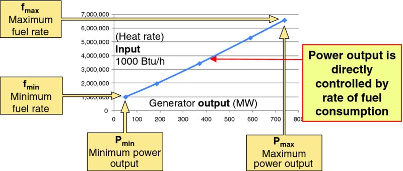
Figure 9.1 Sample Input–Output Curve (copy of Figure 5.7)

The temporal parameters of unit commitment are easily understood via Figure 9.2. After a generator startup cycle completes and the generating unit is operating at its economic minimum power output it is released for economic dispatch so that economic dispatch processes can adjust the unit's power output (between the unit's economic minimum and economic maximum output levels, and subject to the unit's ramp rate). Assume that after the unit's minimum run time it will be shutdown, so the economic dispatch process ramps the unit's power down to economic minimum and then releases the unit for shutdown. After executing the shutdown procedure the unit is offline. Sometime later a unit startup order is issued; it takes the notification time for the generator to connect to the power grid at 0 MW of power output. The unit ramps up from 0 MW to the economic minimum power output in the startup time. When the unit reaches economic minimum power output, the unit is again released for economic dispatch. Minimum downtime is the minimum time between when a unit is released for shutdown and when the unit is back online at economic minimum output and ready for economic dispatch.

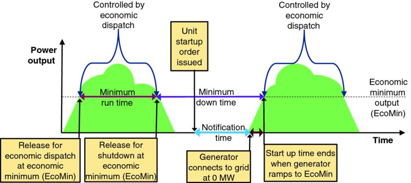
Figure 9.2 Temporal Parameters for Unit Commitment

A commitment plan gives a schedule for starting up and shutting down all power generating equipment. For any arbitrary commitment plan one can estimate both (1) the maximum amount of generating capacity that will be on line at any point in time and (2) the total costs of implementing that plan. By applying appropriate mathematical techniques (e.g., integer linear programming, Lagrangian relaxation) the power industry picks solutions that “maximize social welfare.” A day-ahead plan is constructed as a foundation, and then every 5 minutes (nominally real time in the power industry) that plan is rechecked to fine tune it. Variable and unpredictable patterns of power generation by renewable supplies like solar and wind makes unit commitment and economic dispatch activities more complicated for modern electric grid operators.

9.3 FRAMING THE INFRASTRUCTURE COMMITMENT PROBLEM

The infrastructure commitment problem is somewhat simpler than the unit commitment problem, except for the service drainage problem. Figure 9.3 frames the temporal infrastructure commitment for a single infrastructure element (e.g., a physical server that can be explicitly started up and shut down) with the same graphic as the temporal unit commitment model of Figure 9.2. The Y-axis of Figure 9.3 gives the rough online infrastructure capacity against the X-axis of time. Figure 9.3 explicitly shows power consumed by “infrastructure overhead” as a nominally fixed level during stable operation, and power consumption to serve application loads as variable above that nominally fixed infrastructure overhead. The resources and power consumed by infrastructure overheads will actually vary over time based on infrastructure provisioning and other activities, but this simplification does not materially impact this discussion.

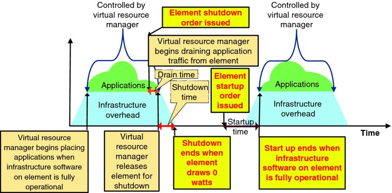
Figure 9.3 Temporal Parameters for Infrastructure Commitment

Let us consider Figure 9.3 in detail across the time window shown:

1. The startup cycle completes for a single target infrastructure element (e.g., a physical server instance that can be powered on and off) when the infrastructure software on that element becomes fully operational and control for allocation and placement of application components onto the element is released to the infrastructure service provider's virtual resource manager.
2. The infrastructure provider's virtual resource manager will allocate virtual resources hosted by online infrastructure servers – including this target server instance – based primarily on:
   1. application component's tolerance of migration or infrastructure drainage action so intolerant application components can be placed onto “always-on” infrastructure elements;
   2. affinity and anti-affinity rules stipulated by application service provider when requesting new resources;
   3. availability of online infrastructure capacity; and
   4. infrastructure service provider's operational policies.
3. At some point an element shutdown order is issued, and this prompts the virtual resource manager to begin draining application traffic from the target element. After drain time, the application workload has been drained, migrated, or deemed expendable, and the virtual resource manager releases the element for hardware shutdown.
4. The infrastructure then initiates an orderly hardware shutdown of the target element. After shutdown time the element is completely powered off and no longer draws any power. Note that the overall shutdown process may include reconfiguration or deactivation of ancillary equipment, such as reconfiguring cooling equipment and disabling networking infrastructure that supports the target element.
5. Eventually an element startup order is issued for the target element. If necessary, ancillary systems for cooling, networking, and power are brought online, and then the target element is energized. After startup time, the infrastructure software on the target node is fully operational and control of the element is released to the virtual resource manager to begin allocating and placing application components onto the target element. The startup cycle is now complete.

The infrastructure commitment problem is thus one of constructing an operational plan that schedules issuing startup and shutdown orders to every controllable element in a cloud data center. As with the power industry's unit commitment problem, the infrastructure commitment problem is fundamentally about picking an infrastructure commitment plan (i.e., schedule of startup and shutdown for all elements in a data center) to assure that sufficient infrastructure capacity is continuously online to reliably serve application workloads at the lowest variable cost. A rough estimate of the available online capacity for an infrastructure commitment plan is the sum of the normal rated capacity of all element instances that are online and nominally available for virtual resource managers to assign new workloads to (i.e., a drain action is not pending on). Both startup and shutdown times for the infrastructure elements are also easy to estimate. The difficulties lie in selecting infrastructure elements that can be drained at the lowest overall cost when aggregate demand decreases. Intelligent placement of virtual resource allocations onto physical elements can simplify this infrastructure drainage problem.

As with the power industry, infrastructure service providers will likely create day-ahead infrastructure commitment plans of when to startup and shutdown each infrastructure element. The infrastructure service provider then re-evaluates the day's infrastructure commitment plan every 5 minutes or so based on actual demand, operational status of infrastructure equipment, and other factors to determine the least costly commitment actions to assure that online capacity tracks with demand, and explicitly issues startup and shutdown orders for target elements.

9.4 UNDERSTANDING ELEMENT STARTUP TIME

Figure 9.4 highlights the startup time of a single infrastructure element in the general temporal context of Figure 9.3. Element startup time varies by equipment type and configuration. This section methodically considers the factors that drive element startup time.

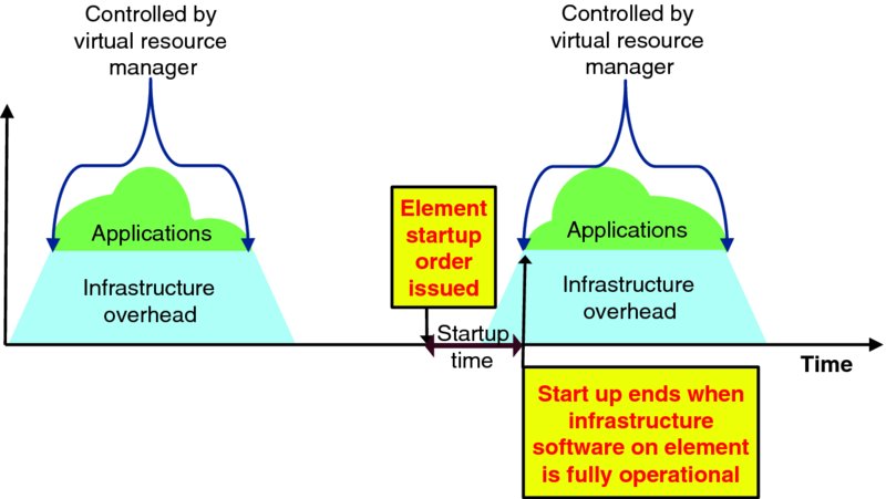
Figure 9.4 Context of Element Startup Time

Element startup begins when the infrastructure service provider's infrastructure commitment operations support system issues an element startup order to the infrastructure management system that controls power for the target element. The startup time includes the following activities:

1. Energize equipment – the target element must be powered on, as well as ancillary equipment that supports the target element. While energizing an individual server may be very fast, if an entire rack of infrastructure equipment was powered off, then one may need to activate cooling and power for the rack, as well as hardware management and monitoring systems and top-of-rack (ToR) Ethernet switches before the first server in the rack can be energized.
2. Power on diagnostic self-tests – firmware boot of many ICT systems includes a power on diagnostic self-test. Large, complex modules can include many complex components so this power on diagnostics often takes many seconds.
3. Boot host operating system – booting host operating system software takes time.
4. Boot infrastructure software on target element – booting a hypervisor, OpenStack and/or other infrastructure platform and management software takes time.
5. Synchronize target element with infrastructure management system – after the infrastructure node is online, it must be fully synchronized with the infrastructure service provider's management and orchestration systems before any of the resources can be allocated to serve application demand.
6. Virtual resource allocation and management system adds target element to the pool of online resources – thereby making the new infrastructure capacity available to serve applications.
7. Element startup time ends – when the new infrastructure capacity is available to be allocated by applications. At this point the infrastructure service provider's virtual resource management system can begin allocating capacity on the target element. Physical throughput limitations will dictate the maximum ramp rate that virtual resources can be allocated and brought into service on the element, and that ramp rate may be impacted by infrastructure demand from the resources already allocated.

Figure 9.5 visualizes the element startup timeline. Note that while Figure 9.3 and Figure 9.4 showed a smooth linear growth in power consumption from 0 W to a higher level when the startup period ends, in reality the element's power consumption is likely to surge as the element is energized, as power on diagnostics access components, as image files are retrieved from persistent storage and executed, and as the element synchronizes with other systems.

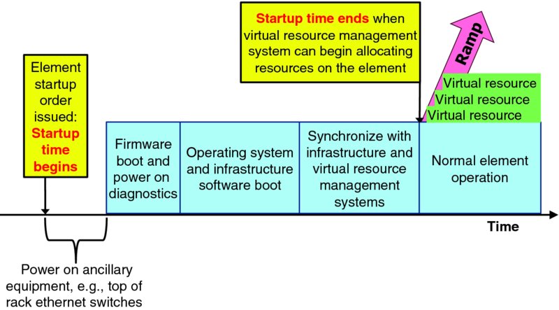
Figure 9.5 Element Startup Time

All power consumed between element startup time begin and startup time end, including power consumed from startup of ancillary equipment until the first element served by that equipment is ready to service allocation requests from the virtual resource management system, contributes to the element's startup cost.

9.5 UNDERSTANDING ELEMENT SHUTDOWN TIME

Figure 9.6 highlights element shutdown in the context of Figure 9.3. At the highest level, element shutdown time is a drain time period when virtual resources are removed from the target element followed by orderly hardware shutdown.

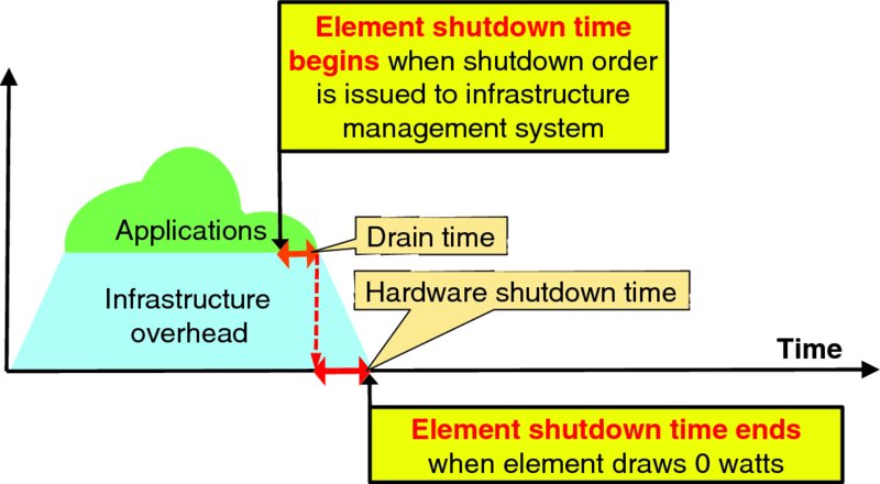
Figure 9.6 Context of Element Shutdown Time

Figure 9.7 visualizes a timeline of the element shutdown process. Before an element shutdown order is issued to a specific element, the infrastructure commitment system must select a specific target to drain; this selection is necessarily completed before the shutdown order can be issued for that target system. Once that shutdown order is issued, the virtual resource manager will embargo the target system so that no further resource allocations will be placed onto that system. The virtual resource manager will then begin methodically draining all application resources currently placed onto the target element. The virtual resource manager has several options to drain each virtual resource:

1. Migrate the resource can be migrated to another infrastructure element
2. Wait for resource to naturally be released with no notification to the application or application service provider
3. Request application and/or application service provider to explicitly drain the resource
4. Suspend the resource (e.g., push a snapshot to disk) without reallocating it to another infrastructure element and then activating it at a later time, possibly on application service provider request
5. Orderly termination of the resource before shutting down the underlying hardware
6. Disorderly termination of the resource by simply forcing a hardware shutdown regardless of the state of the resource

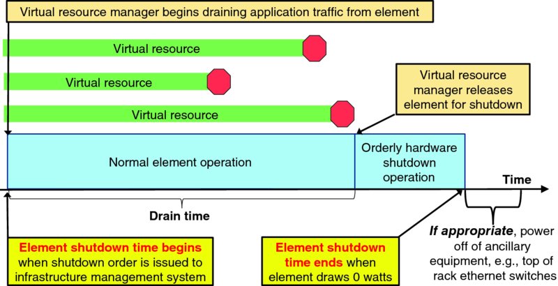
Figure 9.7 Element Shutdown Time

Note that careful planning can potentially shorten and simplify infrastructure drainage actions. With some application knowledge the virtual resource manager could intelligently place particular services onto particular resources to ease/minimize the draining. For example, by keeping track of the average lifetime of particular applications' virtual machines (VMs), one could map short-lived services all onto the same pool of resources, and map long-lived services onto a different pool of resources. This reduces the need of having to migrate or terminate many long-lived services.

Note further that while anti-affinity rules (e.g., do not place both application components A and B into the same infrastructure component failure group) are relatively straightforward to continuously enforce when draining or migrating application components, application affinity rules (e.g., do place application components B and C onto the same infrastructure element) are more problematic because they significantly constrain the choice of destination elements that can accept both B and C simultaneously as well as imply that the migration event must be carefully coordinated to minimize the time that affinity rules are violated. While it is often straightforward to implement affinity rules when allocating resources, it is far more challenging to continuously enforce them when resources are migrated from one infrastructure element to another, or when replacing (a.k.a., repairing) a failed application component instance. Thus, treating affinity rules as advisory rather than compulsory, and thus waiving them when migrating components in the context of lean infrastructure management vastly simplifies lean infrastructure management.

Each of those drain actions has a different completion time, a different impact on user service, and a different burden on the application service provider. Infrastructure service provider policy will likely consider application knowledge when determining which drain action is executed on which resource. Policy will also dictate how long the infrastructure waits for the resource to gracefully drain before taking a more aggressive action, up to disorderly termination, before releasing the element for hardware shutdown.

While the time to complete an orderly hardware shutdown of the target element is likely to be fairly consistent for a particular element configuration, drain times can vary dramatically based on the specific resource instances that are assigned to the target element at the instant that the shutdown order is issued. In particular, drain time is governed by the time it takes for every assigned resource to complete an orderly migration or release, or for infrastructure service provider policy to permit orderly or disorderly termination. Drain time can be estimated as the maximum of the expected drain time for all of the resources placed on the target element at any moment in time. The estimated drain time is driven by the infrastructure service provider's preferred primary, secondary, and tertiary (if used) drain actions for each particular resource, and the timeout period for each action. The selected drain actions are likely to be driven based on the grade of service configured by the application service provider. For example, Table 9.1 offers sample primary, secondary, and tertiary resource drainage policies for each of the four resource grades of service discussed in Section 7.3.3: Create Attractive Infrastructure Pricing Models.

Table 9.1 Sample Infrastructure Resource Drainage Policy

Resource Grade of Service	Primary Drain Action	Secondary Drain Action	Tertiary Drain Action
Strict real time – minimal resource scheduling latency and no resource curtailment	Wait for up to X minutes to drain naturally	Request drainage and wait for up to Y minutes	Migrate
Real time – small resource scheduling latency with occasional and modest resource curtailment is acceptable	Request drainage and wait for up to Y minutes	Migrate	Orderly termination if migration was unsuccessful
Normal – occasional live migration and modest resource scheduling latency and resource curtailment is acceptable	Migrate	Orderly termination if migration was unsuccessful	Disorderly termination if orderly termination was unsuccessful
Economy – workload can be curtailed, suspended, and resumed at infrastructure service provider's discretion	Migrate	Orderly termination if migration was unsuccessful	Disorderly termination if orderly termination was unsuccessful

One can estimate the completion time for each drain action for each resource instance based on throughput and workload on the various infrastructure elements. For instance, one can estimate the time to migrate a resource between two elements based on the size of the resource, the throughput of source, destination, networking, and any other elements involved in the migration action, and other factors. Throughput limitations may preclude the infrastructure service provider from executing all migration actions simultaneously, but the aggregate time for successful migrations of a particular resource load can be estimated. If the migration failure rate is non-negligible, then drain time estimates can include time for a likely number of orderly termination events, and perhaps even disorderly termination events. Likewise the completion time for an orderly or disorderly resource termination can be estimated. Wait and request drain actions are inherently less predictable, so infrastructure service providers may place resources in grades of service that do not gracefully support resource migration onto special servers that are designated as always-on.

As shown in Figure 9.7, if the target element was the last element to be powered off in a chassis, rack, or row of equipment, then it may be appropriate to power off ancillary systems like top-of-rack Ethernet switches, power distribution units, and cooling mechanisms. Infrastructure resources consumed for migration, orderly termination and disorderly termination processes themselves should be charged as drain costs, as well as the target element's infrastructure resources consumed after drain actions begin until the moment that the target element is powered off.

9.6 PULLING IT ALL TOGETHER

Lean infrastructure commitment is best understood in the context of an example. Imagine the hypothetical small scale cloud1 deployment configuration of Figure 9.8 with four racks of infrastructure equipment A, B, C, and D; assume all equipment in each of the four racks can be independently powered on and off. This example considers VM instances; lean management of persistent virtual storage is beyond the scope of this work. Racks A and B are designated as always-on capacity meaning that they will be not regularly be powered off, while Racks C and D are designated as peaking capacity which will be powered on and off on a daily basis to track with demand.

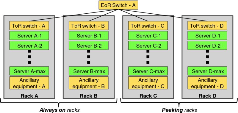
Figure 9.8 Sample Small Cloud

An infrastructure commitment operations support system focuses on scheduling and coordinating the powering up (i.e., committing) equipment in Racks C and D in the morning to track with increasing demand, and powering down (i.e., decommitting) equipment in those racks in the evening as demand rolls off. Since Racks A and B are always-on, the virtual resource manager will place resources that cannot tolerate migration onto those racks, and they will host migratable resources during low usage periods when peaking equipment is decommitted.

Figure 9.9 visualizes the highest level commitment schedule for the sample small cloud of Figure 9.8 for a typical day:

• Rack A is always-on.
• Rack B is always-on.
• Top-of-Rack Ethernet switch (ToR) and ancillary equipment in Rack C along with a minimal economic number of servers is powered on as aggregate demand increases in the early morning.
• Remaining servers in Rack C are powered on just ahead of growing daily demand.
• ToR and ancillary equipment in Rack D along with a minimal economic number of servers is powered on as aggregate demand continues to grow.
• Just enough servers in Rack D (or even Rack C) are committed to meet expected daily demand, so on many days not all of the servers in Rack D (or even Rack C) will be committed.
• In the evening as demand naturally declines on Racks A and B, servers in Racks C and D are embargoed for new resource allocations, thereby beginning the nightly workload roll-off.
• Infrastructure commitment system frequently scans the virtual resource utilization of all servers in Rack C and D, and migrates resources to Rack A and B as the drain costs for each server becomes low enough and space becomes available on always-on equipment. As workload drains from Racks D and C, the servers, ToRs, and ancillary equipments are powered off by midnight.

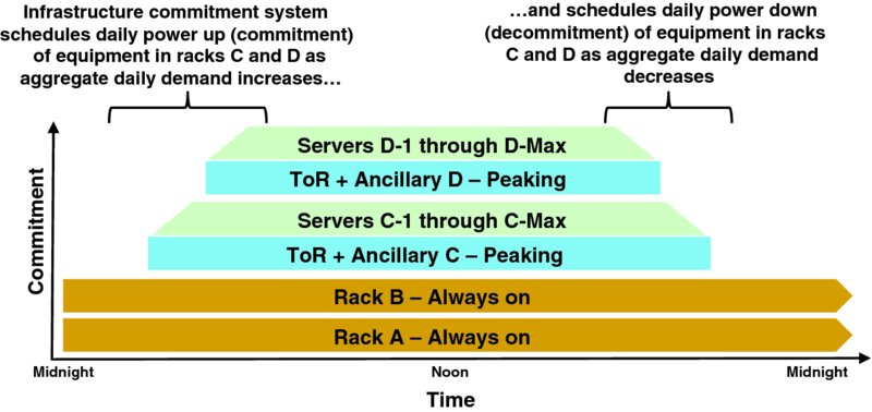
Figure 9.9  Hypothetical Commitment Schedule

Note that the “always-on” equipment will occasional need to be taken offline for maintenance actions like installing security patches. Infrastructure service providers may take advantage of those events to rotate which equipment is “always-on” to level the wear and tear on their infrastructure equipment.

Assume that the infrastructure commitment system executes a decision and planning cycle every 5 minutes 24 hours a day; a summary of key actions across those 5-minute cycles across a hypothetical day might be as follows:

• Midnight – all online virtual resource instances reside on servers in either Rack A or Rack B; Rack C and Rack D are powered off.
• 12:05 am and every 5 minutes thereafter – infrastructure commitment system forecasts aggregate demand for nominally twice the capacity fulfillment lead time. As the next unit of infrastructure capacity growth would be to power up the ancillary equipment in Rack C along with the economically minimum number of servers in Rack C and that is estimated to take 15 minutes, the infrastructure commitment system must decide if the risk of infrastructure demand at 12:35 am exceeding the currently online infrastructure capacity (all of Rack A and Rack B) is non-negligible according to the infrastructure service provider's operational policies. That operational policy will stipulate how much reserve capacity (safety stock) must be maintained at all time based on forecast load, business continuity/disaster recovery plans, and other considerations. Assume this risk is negligible at 12:05 am, 12:10 am, and so on until…
• 4:30 am – forecast aggregate demand at 5:00 am² exceeds the currently online capacity per the infrastructure service provider's minimum online capacity threshold, so the infrastructure commitment system dispatches startup orders for Rack C ancillary equipment, ToR switch, and a minimum economical number of server elements in Rack C.
• 4:45 am – minimum economical number of server instances in Rack C are online and available for the virtual resource manager to allocate. Note that the virtual resource manager will only allocate resources that are migratable onto peaking Racks C or D; resource allocations that cannot tolerate migration, such as strict real-time application components processing bearer plane traffic, will explicitly be placed onto elements in always-on Racks A or B. Further capacity growth actions in Rack C merely require starting up a server (because ancillary equipment and ToR switch are already online), so the infrastructure capacity startup time used by the infrastructure commitment system is now 5 minutes.
• 4:50 am – the infrastructure commitment system forecasts aggregate demand for 10 minutes out (twice the 5-minute startup time for a single server instance in Rack C). As there is sufficient online capacity for 5:00 am, no capacity change action is ordered. 4:55 am, 5:00 am, 5:10 am, 5:15 am forecasts also show acceptable risk, until.

• 5:20 am – the day's demand growth is accelerating and the infrastructure commitment system forecasts insufficient capacity to meet the infrastructure service provider's policy objectives at 5:30 am, so capacity commitment orders are issued for a few more servers in Rack C.

  Meanwhile, the virtual resource manager notices the workload of resources on servers in Racks A and B increases, so the virtual resource manager begins moving migratable workloads off of Racks A and B to underutilized infrastructure capacity in Rack C, and later Rack D. Migratable workloads that resided overnight on always-on servers in Racks A and B can be migrated into peaking capacity on Racks C and D to assure that sufficient capacity to serve the non-migratable workloads that remain hosted by always-on servers in Racks A and B 24/7.

• 5:25 am through 7:00 am – infrastructure commitment system dispatches capacity commitment orders for more servers in Rack C.
• 7:05 am – infrastructure commitment system recognizes that it is exhausting the pool of servers in Rack C that remain to be committed with nominally a 5-minute lead time, so it resets the capacity growth lead time to 15 minutes to account for committing Rack D ancillary equipment, ToR switch, and a minimum economical number of servers.
• 7:15 am – infrastructure commitment system's forecast for 7:45 am demand dictates that Rack D ancillary equipment, ToR switch, and a minimum economical number of servers be committed.
• 7:20 am through 7:30 am – additional servers in Rack C with 5-minute startup time are committed to service
• 7:35 am – minimum economic number of servers in Rack D are online and available to be dispatched by the virtual resource manager and capacity growth lead time reverts to 5 minutes.
• 7:40 am through 4:55 pm – infrastructure commitment server forecast demand 10 minutes into the future and commits additional servers as appropriate.
• 5:00 pm – daily infrastructure decommitment process begins – infrastructure commitment server embargos all committed servers in Rack D which prohibits the virtual resource manager from allocating any additional capacity on Rack D. Thus, workload on Rack D will naturally begin to drain, albeit slowly. During every 5-minute decision cycle the infrastructure commitment server estimates the number of excess server instances online beyond what is necessary to serve actual aggregate demand per the infrastructure service provider's operational policies. If that number is greater than zero, then the infrastructure commitment server scans the virtual resource load assigned to each server instance in Rack C and D and estimates the drain cost and time for each server instance. Starting with the server instance with the lowest estimated drain cost, the infrastructure commitment server verifies that the economic benefit of immediately decommitting that server outweighs the cost of draining it. If the decommitment benefits sufficiently outweigh the current drain costs, then the infrastructure commitment system dispatches a shutdown order for that server instance. The infrastructure commitment system will repeat the drain cost/benefit comparison for servers in Racks C and D in increasing order of drain costs until either the cost/benefit tradeoff is no longer favorable or sufficient servers are earmarked for shutdown.
• 5:05 pm and every 5 minutes thereafter – infrastructure commitment server determines which, if any, server instances in Rack C and D can be cost effectively decommitted. As both application and aggregate infrastructure demand rolls off through the evening, the drain cost and drain times should decrease so it should be easier to select servers to decommit. The infrastructure commitment server is biased to drain one of the peaking racks first; let us assume Rack D. When the number of committed servers on Rack D falls below the minimum economic number, the workload on the remaining servers will be drained and shutdown so that Rack D can be fully decommitted.
• 8:00 pm – Rack C is embargoed so the virtual resource manager will no longer allocate new resources on any server in Rack C to minimize the number of resources that will need to be migrated over the next few hours.
• 8:50 pm – number of committed servers on Rack D falls below the economic minimum number, so remaining resources are drained by migrating resources to always-on servers in Racks A and B.
• 11:05 pm – number of committed servers on Rack C falls below the economic minimum number, so remaining resources are migrated to Racks A and B, then remaining servers on Rack C are decommited, ToR-C, and ancillary equipment are powered off.
• Midnight – all online virtual resource instances reside on servers in either Rack A or Rack B; Rack C and Rack D are powered off.

As migration events consume infrastructure resources and inconvenience the impacted application service provider, infrastructure service providers will set policies with some hysteresis that balances power savings against overhead costs and application service provider impact. Setting a policy of not normally migrating any virtual resource more than twice a day (e.g., hosted overnight/off-peak on always-on equipment and hosted in peak periods on peaking equipment) may be a reasonable balance of controllability for the infrastructure service provider and minimal inconvenience for the application service provider. Compelling discounts or policies can entice applications to willingly support occasional and impromptu (i.e., without prior notification) resource migration by the infrastructure service provider will vastly simplify aggressive infrastructure commitment operations. Beyond pricing policies attractive enough for application service providers to opt-in to voluntarily support migration (and perhaps other drainage actions), infrastructure service providers must assure that the migration actions:

• Have consistent, limited (and hopefully minimal) impact on user service – resource stall time per migration event should be brief; ideally the infrastructure service provider will establish quantitative service level objectives for the maximum acceptable stall time during a migration event.
• Are highly reliable – as migration events will nominally occur twice a day for each resource instance that persists for more than 24 hours, they will be routine and thus should be extremely reliable. Assuming twice daily resource migration events, 99.999% reliable converts to a mean time between migration failures (MTBF) of 137 years per resource.³
• Automatically recover application service in the event of failure – to minimize application service provider expense/burden if an infrastructure-initiated drainage action failed.
• Are acceptably infrequent. Clear expectations and limits on the frequency of drainage events should be set to minimize overall user service impact and application service provider burden. For example, infrastructure service providers might commit to not migrating a resource for power management reasons more than twice a day.

Note that since servers in always-on racks A and B will have more simultaneous – and presumably lightly used – VM instances than the peaking elements in Racks C and D, the servers in Racks A and B might be configured differently from the servers in Racks C and D, such as being equipped with more RAM to efficiently host a larger number of lightly used VM instances in off-peak periods than peaking servers are likely to experience.

9.7 CHAPTER REVIEW

• ✓ Infrastructure commitment optimization principles can usefully be adapted from the power industry to optimize power management of cloud service providers' physical infrastructure capacity to achieve the goal of lean cloud computing: sustainably achieve the shortest lead time, best quality and value, highest customer delight at the lowest cost, as well as reducing electricity consumption and hence carbon footprint.

NOTES

1 While many readers associated massive, warehouse scale regional data centers with cloud computing, cloud infrastructure can also be distributed to metropolitan and local facilities, including enterprise locations and even collocating cloud infrastructure with wireless base stations or wireline access equipment to provide the lowest possible user service latency or for other reasons.

² 5:00 am is 30 minutes after the then current time of 4:30 am; 30 minutes into the future is twice the 15-minute startup time of the next unit of infrastructure capacity to be committed, which is rack C ToR, ancillary equipment and a minimum economic number of servers.

³ 99.999% reliable means 0.001% of migration events fail, or 1 in 100,000 migration actions. Assuming two migration events per resource per day, that is 1 failure in 50,000 resource-days. Dividing 50,000 resource-days by 365.25 days per average year yields 136.9 years per resource.