Chapter 7
Tidal mixing
We saw in the last chapter how internal tide waves mix the interior of the deep ocean. In this chapter, we describe some important examples of tidal mixing in shelf seas, where the water is shallow and tidal currents can be much faster than in the deep ocean.
Turbulence and mixing
Most of the energy lost from the tide through friction is first converted into turbulence: a random movement that can be seen when watching water flow. In some places the flow is fast and in others slow; there may be places where the water moves in the opposite direction to the main flow. These variations in speed are caused by eddies: swirls of water added to the mean current. The largest eddies fill the space available: the width or the depth of a channel. They break down into smaller eddies, and then smaller ones again, down to the smallest eddies in which the tide’s energy is ultimately dissipated as heat. This cascade of turbulent eddies of different sizes was memorably described by the British polymath Lewis Fry Richardson:
Big whirls have little whirls which feed on their velocity, and little whirls have lesser whirls and so on to viscosity.
One of the most obvious manifestations of marine turbulence is the great swirl of a tide-generated whirlpool or maelstrom. Maelstroms are often associated with narrow, tidal sea straits, between islands, for example. Differences in tidal elevation at the ends of the strait create surface slopes which drive fast ‘hydraulic’ currents through the strait. Where such a current emerges from the strait and interacts with other currents or topographic features, areas of lateral current shear occur and eddies, or vortices, may develop.
The whirlpool (or mythological sea monster) Charybdis terrified the ancients, as recounted by Homer in The Odyssey. It is sometimes linked with the modern-day Garofalo feature of the Strait of Messina, between Italy and Sicily. The Moskstraumen maelstrom off the Lofoten Islands in Norway is mentioned in old Norse poems and on nautical maps, and features in Edgar Allan Poe’s ‘A Descent into the Maelstrom’, Jules Verne’s Twenty Thousand Leagues under the Sea, and Herman Melville’s Moby Dick. Some maelstroms can be very striking (Table 5), but over the years authors and artists have tended to exaggerate somewhat (see Figure 32). The largest ones are certainly not sensible places to take a small vessel at peak flow, but the origins and dynamics of large whirlpools remain poorly understood.
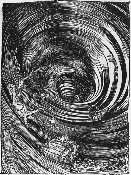
32. An illustration of a tidal whirlpool or maelstrom by Arthur Rackham (1867−1939).
Table 5. (In)famous tidal whirlpools or maelstroms
| Whirlpool/maelstrom | Location |
|---|---|
| Saltstraumen | Strait connecting Saltfjord and Skjerstadfjord, near Bodø, Norway |
| Moskstraumen | Between the islands of Moskenesøya and Mosken, Lofoten Archipelago, Norway |
| Corryvreckan | Between the islands of Jura and Scarba, Scotland |
| Naruto | Between Naruto (Tokushima) and Awaji Island, Japan |
| Old Sow | Between Deer Island (New Brunswick, Canada) and Moose Island (Maine, USA) |
The size of the smallest eddies—the scale at which the energy is ultimately dissipated as heat—was determined by the Russian mathematician Andrey Nikolaevich Kolmogorov using dimensional analysis. The Kolmogorov Scale depends on the molecular viscosity of the fluid (seawater in our case) and the rate at which the turbulent energy is dissipated. For tidal flow in shallow water it is possible to get a good idea of this second quantity. The frictional force depends on the square of the flow speed and the energy dissipation rate on the cube of the speed. For a tidal current of 1 metre per second in water 20 metres deep, for instance, the energy dissipation rate is 0.00125 watts per kilogram of water and the Kolmogorov Scale is 0.3 millimetres. If the flow increases to 2 metres per second in the same depth of water, the Kolmogorov Scale is reduced to less than 0.2 millimetres. Increasing tidal energy creates eddies which can squeeze into smaller spaces.
Turbulent eddies make a very effective mixing mechanism. One way to visualize how this happens is to imagine two adjacent volumes in the sea which, every second, exchange some of their water. Water properties, such as temperature or salinity, will also be exchanged and any differences between the two volumes will be smoothed out over time. Alternatively, we can imagine two small parcels of water initially close together being carried along by the mean flow. Because of the turbulence, they will not follow the same path exactly; the parcels will move apart as time goes on. One hundred such parcels starting close together will spread out, or diffuse, into the surrounding water.
Heat storage in the sea
An important example of mixing by the tide is the downward stirring of the Sun’s heat. The sea is a great store of heat: water has a large thermal capacity and the heat stored in summer is released in winter, smoothing out the seasons. To maximize the storage, the heat needs to be mixed down. Unlike the atmosphere (which is warmed mainly at the bottom, where it touches the ground) seas are warmed at the surface. It takes energy to mix the warm, buoyant surface waters down into the colder and denser water below. In shelf seas, the principal source of this energy is the turbulence made by the wind rubbing on the sea surface and the tide rubbing on the seabed.
We can use an energy argument to work out how deep the tides can mix the Sun’s heat. If water of depth d (from surface to bottom) is warmed and mixed so that the temperature remains uniform throughout, thermal expansion will raise the centre of gravity and the potential energy will increase at a rate proportional to the heating rate times d. This extra potential energy is provided by the turbulence. The rate at which tides create turbulent energy is proportional to the cube of the current speed, u3. We can imagine that a proportion of this tidal turbulent energy is converted to potential energy as it mixes heat down. If this proportion (and the heating rate) is constant then the maximum depth of water that can be mixed by the tide, dmax, will be proportional to u3. Observations confirm this idea and suggest that dmax in metres is about 70u3 if u is measured in metres per second at spring tides. This allows us to calculate the proportion of the tide’s turbulent energy used for the vertical mixing of heat; it is about 0.5 per cent.
Tidal currents with maximum speed 1 metre per second are therefore capable of maintaining mixed conditions, in a mid-latitude summer, in water depths up to 70 metres. A small increase in current speed to 1.13 metres per second will mix heat down to the bottom in 100 metres of water. The most vigorously stirred shelf region that we have visited is the north channel of the Irish Sea, lying between Northern Ireland and Scotland. Here, mixed conditions are maintained all year in depths over 200 metres. Because mixing heat downwards keeps the surface cool, less heat is lost to the atmosphere. The summer heat stored in these deep mixed waters is about twice that in water without tidal stirring, a fact that must contribute to the mild winters experienced in this region.
Tides and the weather
It is sometimes possible to see, directly, the effect of tidal mixing on the temperature of the sea. Figure 33 shows the tidal curve and water temperature in winter at a coastal site in North Wales. There is a variation of temperature in phase with the spring–neap tidal cycle (the fortnightly cycle of temperature is much more pronounced than the small daily changes). The water at spring tides is nearly 2 degrees Celsius warmer than at neaps.
33. Variation of water temperature and depth in the Menai Strait, North Wales.
Observations like this are intriguing because they are hard to explain. Why should the water be warmer at spring tides? A likely explanation is that the flood tide brings, in winter, warmer offshore water to the coast, where it mixes with coastal water and raises its temperature. The effect will be greatest at spring tides because a greater volume of offshore water will be added to the mixture. If this is correct, we would expect the effect to reverse in summer when the deeper offshore waters are cooler than coastal water, and this is indeed what happens. This explanation may not be the whole story though; it is possible that local effects, involving the phase of the tide relative to the daily variation of solar heating, are also important.
Even without a full explanation of the observations in Figure 33, the fact remains that coastal water temperature can change with the spring–neap tidal cycle. If the water temperature is varying in this way, then air temperature (and possibly other meteorological parameters, such as the wind) will tend to follow suit. Experienced seafarers that we have spoken to are convinced that there are links between the tides and the weather.
Tidal mixing fronts
In parts of the shelf where the tides are not strong enough to mix the Sun’s heat right down to the seabed, the water in summer becomes stratified. A surface layer warmed by the Sun and stirred by the wind lies over a deeper, cold layer, the two separated by a vertical gradient of temperature called the seasonal thermocline.
Shelf seas at temperate latitudes in summer are divided into regions which are stratified and those which are vertically mixed, depending on the strength of the tidal streams and the depth of water. The transition from one to the other happens rapidly and creates a structure called a tidal mixing front (see Figure 34). On one side of the front, the water is stratified; on the other it is vertically mixed with an intermediate ‘cool’ temperature. The depth of water at the front is the maximum depth that can be mixed by the tide, and so, in metres, is about seventy times the cube of the spring current (in metres per second) at the front.
34. A tidal mixing front.
Tidal mixing fronts have been found on most of the continental shelves known to have large tides, including the Patagonian Shelf in South America, George’s Bank in Canada, Cook Strait in New Zealand, and the north-west European Shelf. Unlike weather fronts in the atmosphere, tidal mixing fronts form in the same place each year. The fronts form in early spring as the stratification forms, remain in place throughout the summer, and then gradually retreat into deeper water in the autumn as surface heating is reduced and winds pick up.
We have learned much about the behaviour of tidal mixing fronts from satellite data. Satellites equipped with infra-red sensors are able to pick out the temperature contrast between the warm surface of the stratified water and the relatively cool mixed water.
The fronts are known for their biological productivity. They create favourable conditions for the growth of phytoplankton, the microscopic algae which are the base of the marine food chain. Photosynthesis and the growth of phytoplankton are usually limited by the supply of either sunlight or nutrients (their other requirements, carbon dioxide and water, are plentiful in the sea). In the stratified parts of shelf seas, the plankton strip the nutrients out of the surface layer during their spring growth ‘bloom’; the bottom layer (which has plenty of nutrients left) is too dark for them. Growth then slows down in the stratified water (it never really gets going in the mixed water because the phytoplankton, mixed from surface to bottom, receive too little light averaged over a day). Near a tidal mixing front, nutrients from the mixed side of the front can be transferred across into the surface layer of the stratified water, sustaining phytoplankton growth.
One mechanism for transferring material across a tidal front is the fortnightly variation of tidal energy associated with the spring–neap cycle. At neap tides, tidal mixing is reduced and some of the mixed water next to the front becomes stratified; as this happens nutrients from the mixed side of the front become trapped in the newly formed stratified water. Other material is mixed across as the fronts advance and retreat with a fortnightly cycle. Oxygen is depleted in the bottom layer by respiration. Instruments on marine gliders have recently detected a twice-monthly variation in oxygen concentration in the bottom layer of the stratified water close to a front in the Irish Sea, presumably created as water from the mixed side of the front (rich in oxygen because it is in contact with the atmosphere) is transferred across the front at a neap tide.
Muddying the waters
Tidal currents flowing over the seabed lift sediment particles, in large numbers, and mix them up towards the surface. The result is that tidal waters are often cloudy and opaque, no great encouragement for a dip in the sea. Observations of the particles under a microscope show that they are a mixture of flakes of mud and small living and dead organisms. Different kinds of particle stick together in clumps called aggregates or flocs, bound by biogenic polysaccharide glue. The aggregates are denser than water and tend to sink gradually towards the seabed. The Irish physicist George Gabriel Stokes showed that the sinking speed of a particle in water depends on the square of its diameter. Large flocs will settle out of suspension more quickly than individual particles.
These denser-than-water particles can be held in suspension in the sea by turbulence. The process is analogous to the downward mixing of heat: in both cases work needs to be done against gravity. We can again use an energy argument to work out how much material the tide can hold in suspension. The energy needed per unit time depends on the product of the particle concentration c and the settling speed w. If a fixed fraction of the total energy dissipated by the tide (proportional to u3) is used to hold the particles up, then the concentration c will be proportional to u3/w.
This idea can be tested using observations from satellites. The particles near the sea surface scatter sunlight, some of which makes it back out through the atmosphere and, remarkably, can be picked out by satellite instruments. Figure 35 shows an image of light scattered by particles in the Irish Sea. The areas of high ‘brightness’ (and particle concentration) marked A, B, and C are also areas of strong tidal streams—M2 surface currents peak at more than 1 metre per second at each of these places. In fact, with the exception of some small areas of high turbidity associated with river input, the distribution of suspended particles in the Irish Sea closely matches the distribution of tidal current speeds.

35. Brightness of the Irish Sea measured from space. Lighter shades correspond to brighter waters.
In principle, the relationship between suspended particle concentration and tidal energy can be used to estimate particle settling speed, an important but difficult-to-measure parameter. Recent observations have shown that the settling speed is greater in summer than in winter. This finding is consistent with greater particle aggregation in summer when biological ‘stickiness’ is more active.
Isolated turbidity maxima
The patches of muddy water associated with fast tidal currents, labelled A−C in Figure 35, present something of a puzzle. There is no obvious source of fine sediments to maintain these isolated turbidity maxima, as they are called. The seabed is composed of pebbles, mostly, and there are no large rivers nearby. Without a local source, the particles in the maxima will diffuse away, down the concentration gradient into the surrounding water. A similar thing would happen if, say, a passing tanker were to discharge a cargo of ink at one of these sites. The ink would initially colour the water but then mix with its surroundings, become diluted, and eventually disappear. The satellite pictures, however, tell us that the turbidity maxima are always present despite the absence of an obvious source.
The answer to this puzzle relies on the fact that flocculated particles can change their size with the tide. This happens because the flocs are too frail to withstand the disrupting effects of turbulence. The upper limit for the size of a marine floc is the size of the smallest turbulent eddies—the Kolmogorov Scale. If the tidal currents increase and the turbulent scale decreases, the size of the flocs is reduced.
Within the strong currents of a turbidity maximum the flocs are small and easily held up near the sea surface where they scatter sunlight. These small flocs diffuse out of the maximum into the less turbulent surrounding water where the Kolmogorov Scale is greater. Here, the flocs grow in size (this happens by particles colliding and sticking together). The larger flocs created around the edge of the maximum now diffuse down the concentration gradient of large flocs, that is back into the maximum, where they are torn up into small flocs and the cycle continues.
This interpretation of the processes happening in isolated turbidity maxima has been confirmed by observations on the edge of the maximum marked A in Figure 35. These have shown that, averaged over a tide, there is a flux of large particles entering the maximum and a balancing flux of smaller ones leaving.
Tidal mixing in estuaries
Estuaries are places where salt and fresh water mix (this is true in most cases. There are estuaries in hot, dry countries where there is little fresh water available. In these inverse estuaries, the water becomes hyper-saline and processes are somewhat different). In regular estuaries with small tides, the circulation is controlled mostly by the fact that salt water is a few per cent denser than fresh water. River water entering the estuary flows over the top of salt water that has come in from the sea. A two-layer system is formed, with an interface, called the halocline, separating the layers. As river water flows seaward at the surface it pushes against the lower layer, which takes on the form of a wedge of salt water protruding into the estuary along the bottom. These salt wedge estuaries are found in places where the tides are small; an example is the Mississippi River in the United States.
In shallow estuaries with moderate tides, turbulence generated by tidal streams (and winds) mixes water vertically between the layers and the estuary is classified as partly mixed. The halocline becomes blurred and the difference in salinity between the layers is reduced. Because the outward-flowing surface layer is now partly salt water, a greater volume of water flows seaward to remove the river water. For example, if a volume V of river water enters the estuary in a day and mixes with an equal volume of seawater, then a volume 2V of the mixture must leave the estuary. In this case, mixing doubles the surface flow. To maintain the volume of water in the estuary there is also a flow (of volume V per day) of salt water inland along the bottom. This two-way flow is a characteristic of partly mixed estuaries and is called the estuarine circulation. Partly mixed estuaries are common in places with medium tides. For example, many large estuaries in northern Europe are partly mixed.
In an estuary with very large tides, the layering is destroyed completely and the estuary becomes well-mixed in the vertical with no discernible difference in salinity from surface to bottom. The estuarine circulation continues but now the rapid exchange of parcels of water between the surface and bottom slows down the horizontal flow in both directions. The effect is similar to that in the entrance to a theatre when people are leaving after a show and the next audience is coming in. As long as things are organized with people leaving the door on one side and entering on the other, the exchange can proceed smoothly. But if some people now start stepping sideways across the doorway, taking their momentum with them, the motion becomes confused and the exchange slows down. In a well-mixed estuary, the vertical exchange of horizontal momentum has the effect of increasing the stickiness or viscosity of the water and slowing down the horizontal flows.
The effect of bottom and side friction on the tide creates other effects in estuaries. On the flood tide, when water flows into the estuary, the faster currents at the surface carry salt water from the sea over the top of fresher water in the estuary. Because salt water is denser, this is an unstable situation. The salt water sinks, creating convection currents which add to the turbulence. In contrast, on the ebb, the faster surface currents push fresh water over salt water. This is gravitationally stable and the water can become stratified at this time. The temporary stratification created by the action of vertically sheared currents on a horizontal salinity gradient is known as tidal straining.
In well-mixed estuaries during the flood tide, a foam line can sometimes be seen running along the middle of the estuary (Figure 36(a)). This foam line is caused by the flood tide being slowed down by friction with the sides of the estuary. The flood current flows fastest along the central axis of the estuary. In a cross-section of the estuary during the flood, the salinity is greatest at a point in the middle at the surface. The denser salt water at this point sinks and is replaced by water flowing in from the sides (Figure 36(b)). The currents converging on the centre line carry floating material which accumulates to make the foam line, or axial convergence.
36. (a) A foam line down the middle of a well-mixed estuary on the flood tide; and (b) a sketch of the process creating the axial convergence.
The presence of the secondary circulation at right angles to the main flow can be demonstrated by placing a line of floats across the estuary (F to F’ in Figure 36). The floats are carried upstream by the flood tide but at the same time converge on the centre line. This simple measurement enables the speed of the secondary circulation to be determined. It is surprisingly fast—up to one quarter of the speed of the main flood current. When the current turns to ebb, the secondary circulation stops and the axial convergence disappears.
Harnessing the tide
People living by the sea quickly learned to take advantage of the special opportunities that tides provide. An early example was the construction of fish traps: walled enclosures which filled with seawater (and fish) as the tide came in. In the Middle Ages in Europe, tide mills used the power of tidal streams to make flour for bread. Some of these mills still exist and are interesting places to visit.
Today, the emphasis is on using the tide to generate electricity. A number of tidal power plants are in operation worldwide and the use of the tide in this way is likely to grow. Countries with large tides have the potential to generate a significant proportion of their energy needs if the tide can be harnessed effectively.
Tides can be used to make electricity in a number of ways. One is to make a dam across the mouth of an estuary or bay. The tide flows in and out of the estuary through a turbine in the dam; the turbine is connected to a generator and electricity is produced. The power output of such a scheme depends on the square of the tidal range (since the potential energy released depends on the mass of water and the height of the centre of gravity, both of which are proportional to the range of the tide). Places with a large tidal range, such as the Severn estuary in the UK, are preferred sites for tidal dams. There is an environmental cost to schemes like this, however. The dam raises the mean water level inside the estuary and mudflats, important feeding grounds for birds, become permanently submerged.
Alternatively, electricity can be made by placing a turbine and generator directly into a fast flowing tidal stream. Some clever ideas have been proposed for maximizing the energy that can be extracted. One is a tethered glider which soars backwards and forwards at right angles to the flow (like a kite in the wind), increasing the speed at which the water flows through the turbine. Tidal stream turbines in a semi-diurnal tide will have peak generation four times a day, at times of maximum flood and ebb. They can be placed in positions around the coast such that the different phases of the tide produce electricity continuously over twenty-four hours.
Innovations in using tidal energy are encouraged by local needs and initiative. In Mozambique, students at the School of Coastal Marine Science are required to design, build, and operate a turbine to generate a small amount of electricity. The simplest rotor design has a vertical axis between curved blades making an ‘S’ shape viewed from above. This design, a Savonius rotor, always presents one concave and one convex blade to the flow, and since the drag is greater on the concave blade, the rotor turns at a speed which depends on the difference in the drag on the blades.
When a dynamo is attached to the turbine, something interesting happens. The dynamo can be driven by a loop of rope passed around the rotor. Power generation is equal to the product of the tension in the rope W (called the ‘load’, and set by the specification of the dynamo used) and the speed v with which the rope moves. However, the load and the rotor speed are inversely related to each other. A light load allows the rotor to turn quickly, but generates little power because W is small. Too much load also generates little power because the rotor turns slowly and v is small. There is an optimum load which produces the maximum value of Wv and generates the most electricity (Figure 37).
37. Power output (continuous line) and rotor speed (dashed) for a small tidal electricity plant.
For the turbine in Mozambique, which is 2 metres across and 2 metres high placed in a tidal river with maximum currents of 1 metre per second, the optimal power output is 100 watts every six hours. It’s not much, but it is enough to charge batteries for a back-up power supply.