Probability and random variables are an integral part of computation in a graph-computing platform like PyTorch. Understanding probability and associated concepts are essential. This chapter covers probability distributions and implementation using PyTorch, and interpreting the results from tests.
In probability and statistics, a random variable is also known as a stochastic variable , whose outcome is dependent on a purely stochastic phenomenon, or random phenomenon. There are different types of probability distributions, including normal distribution, binomial distribution, multinomial distribution, and Bernoulli distribution. Each statistical distribution has its own properties.
The torch.distributions module contains probability distributions and sampling functions. Each distribution type has its own importance in a computational graph. The distributions module contains binomial, Bernoulli, beta, categorical, exponential, normal, and Poisson distributions.
Recipe 2-1. Sampling Tensors
Problem
Weight initialization is an important task in training a neural network and any kind of deep learning model, such as a convolutional neural network (CNN), a deep neural network (DNN), and a recurrent neural network (RNN). The question always remains on how to initialize the weights.
Solution
Weight initialization can be done by using various methods, including random weight initialization. Weight initialization based on a distribution is done using uniform distribution, Bernoulli distribution, multinomial distribution, and normal distribution. How to do it using PyTorch is explained next.
How It Works
To execute a neural network, a set of initial weights needs to be passed to the backpropagation layer to compute the loss function (and hence, the accuracy can be calculated). The selection of a method depends on the data type, the task, and the optimization required for the model. Here we are going to look at all types of approaches to initialize weights.
If the use case requires reproducing the same set of results to maintain consistency, then a manual seed needs to be set.
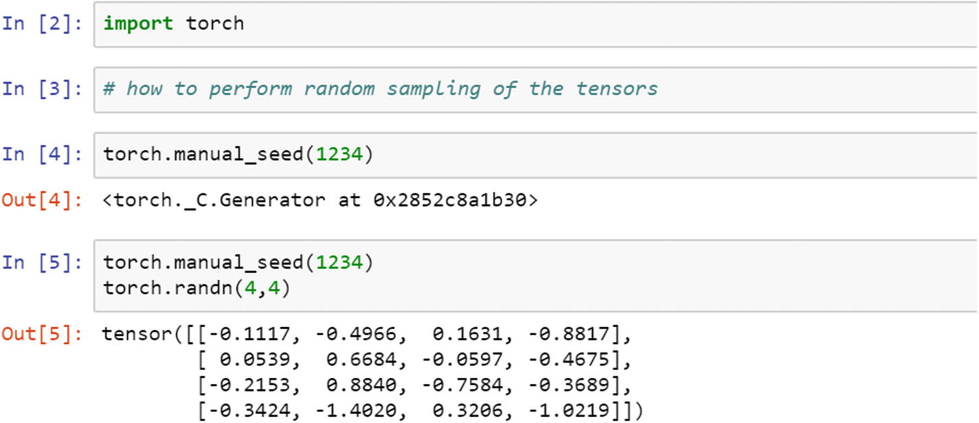

The function of x has two points, a and b, in which a is the starting point and b is the end. In a continuous uniform distribution, each number has an equal chance of being selected. In the following example, the start is 0 and the end is 1; between those two digits, all 16 elements are selected randomly.

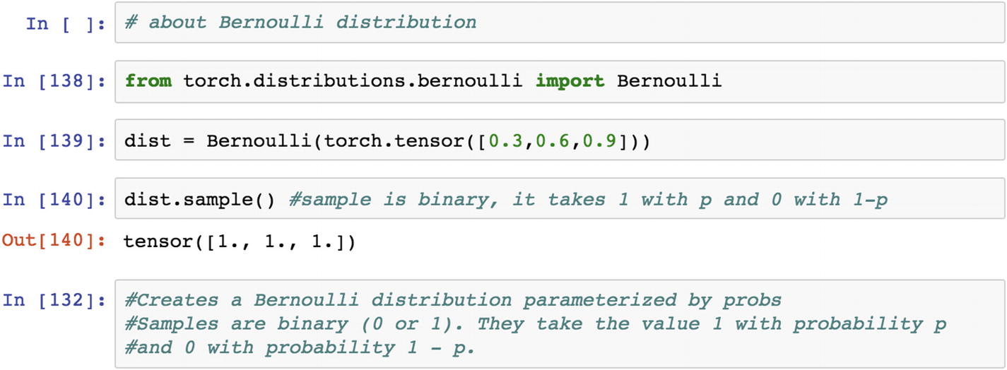
In statistics, the Bernoulli distribution is considered as the discrete probability distribution, which has two possible outcomes. If the event happens, then the value is 1, and if the event does not happen, then the value is 0.

From the Bernoulli distribution, we create sample tensors by considering the uniform distribution of size 4 and 4 in a matrix format, as follows.

The generation of sample random values from a multinomial distribution is defined by the following script. In a multinomial distribution, we can choose with a replacement or without a replacement. By default, the multinomial function picks up without a replacement and returns the result as an index position for the tensors. If we need to run it with a replacement, then we need to specify that while sampling.

Sampling from multinomial distribution with a replacement returns the tensors’ index values.

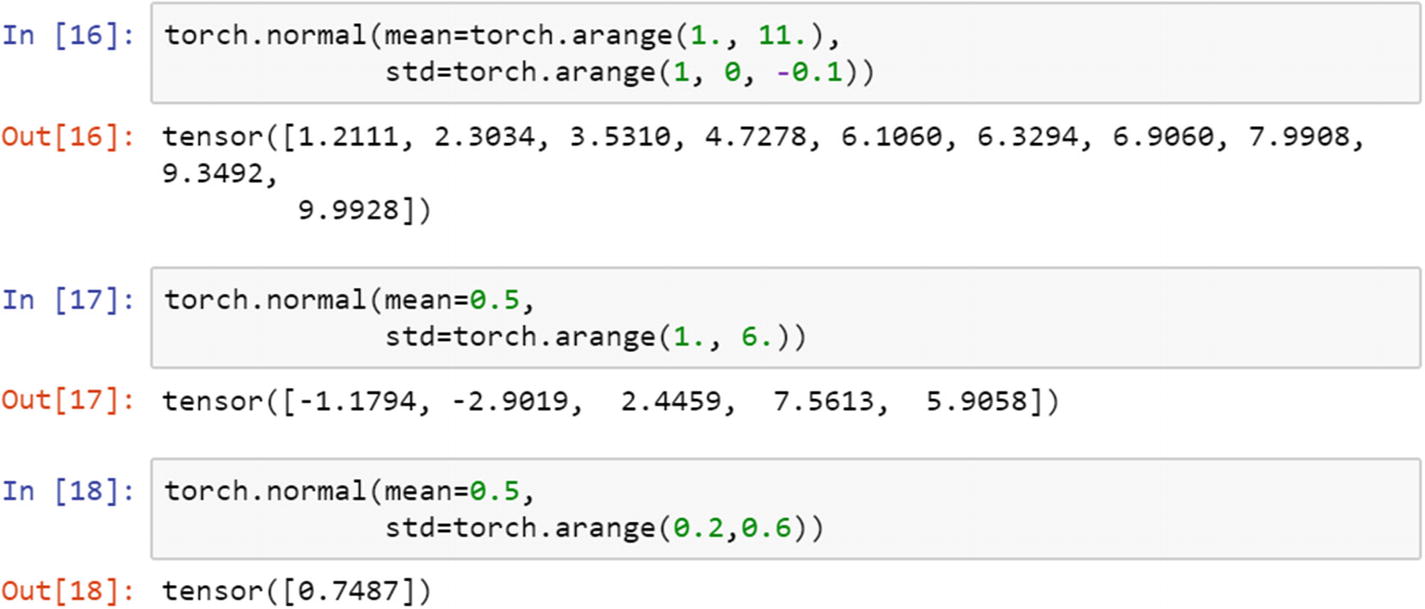
The weight initialization from the normal distribution is a method that is used in fitting a neural network, fitting a deep neural network, and CNN and RNN. Let’s have a look at the process of creating a set of random weights generated from a normal distribution.
Recipe 2-2. Variable Tensors
Problem
What is a variable in PyTorch and how is it defined? What is a random variable in PyTorch?
Solution
In PyTorch, the algorithms are represented as a computational graph. A variable is considered as a representation around the tensor object, corresponding gradients, and a reference to the function from where it was created. For simplicity, gradients are considered as slope of the function. The slope of the function can be computed by the derivative of the function with respect to the parameters that are present in the function. For example, in linear regression (Y = W*X + alpha), representation of the variable would look like the one shown in Figure 2-2.
Basically, a PyTorch variable is a node in a computational graph, which stores data and gradients. When training a neural network model, after each iteration, we need to compute the gradient of the loss function with respect to the parameters of the model, such as weights and biases. After that, we usually update the weights using the gradient descent algorithm. Figure 2-1 explains how the linear regression equation is deployed under the hood using a neural network model in the PyTorch framework.
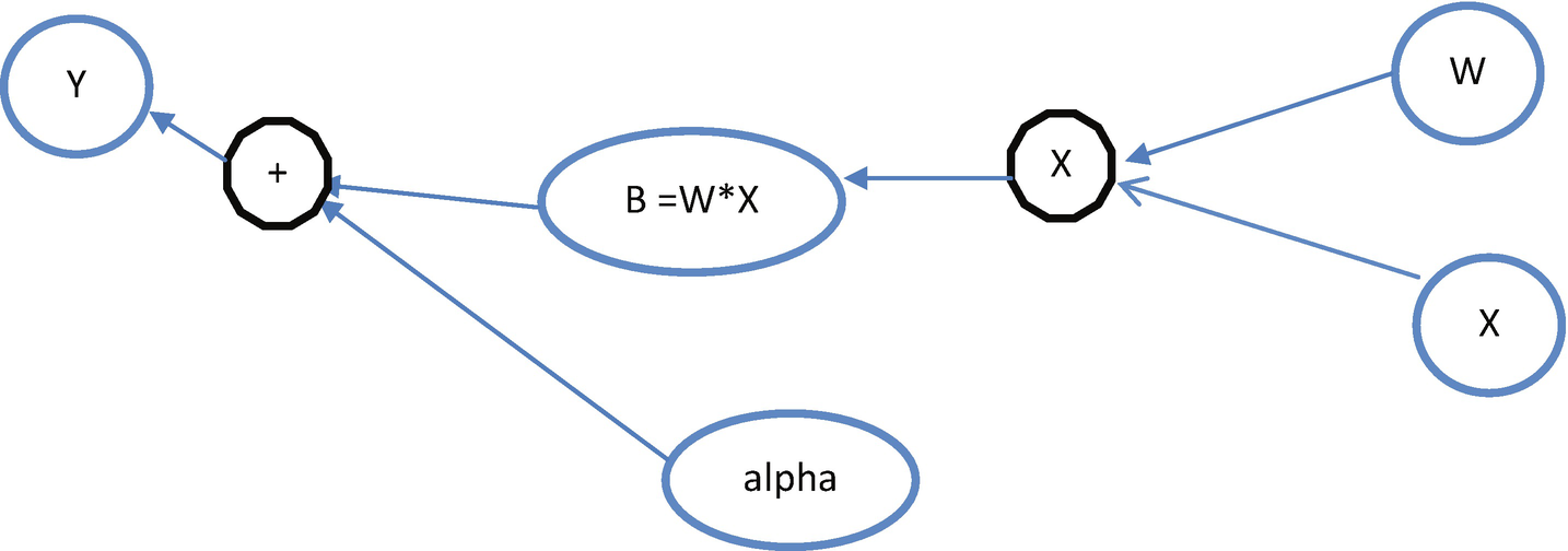
A sample computational graph of a PyTorch implementation
How It Works
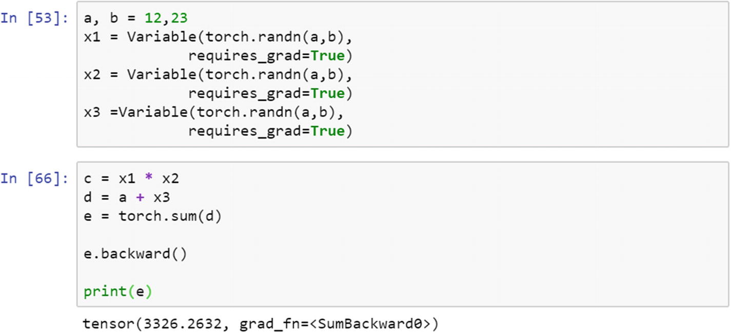
An example of how a variable is used to create a computational graph is displayed in the following script. There are three variable objects around tensors— x1, x2, and x3—with random points generated from a = 12 and b = 23. The graph computation involves only multiplication and addition, and the final result with the gradient is shown.
The partial derivative of the loss function with respect to the weights and biases in a neural network model is achieved in PyTorch using the Autograd module. Variables are specifically designed to hold the changed values while running a backpropagation in a neural network model when the parameters of the model change. The variable type is just a wrapper around the tensor. It has three properties: data, grad, and function.

Recipe 2-3. Basic Statistics
Problem
How do we compute basic statistics, such as mean, median, mode, and so forth, from a Torch tensor?
Solution
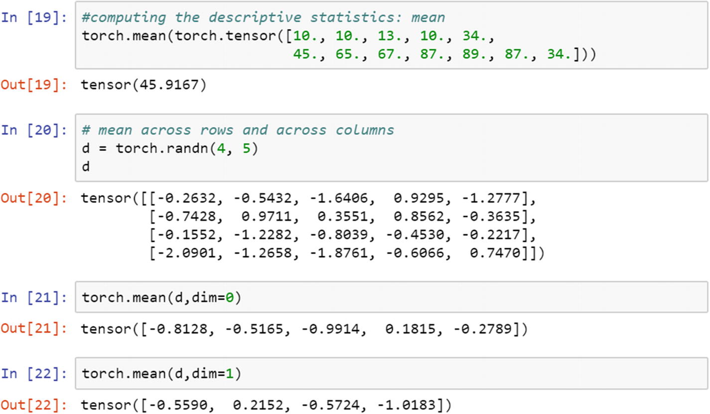
Computation of basic statistics using PyTorch enables the user to apply probability distributions and statistical tests to make inferences from data. Though the Torch functionality is like that of Numpy, Torch functions have GPU acceleration. Let’s have a look at the functions to create basic statistics.
How It Works
The mean computation is simple to write for a 1D tensor; however, for a 2D tensor, an extra argument needs to be passed as a mean, median, or mode computation, across which the dimension needs to be specified.
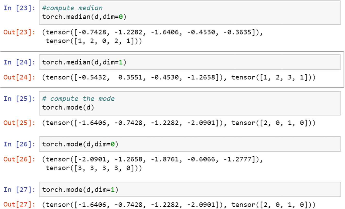
Median, mode, and standard deviation computation can be written in the same way.
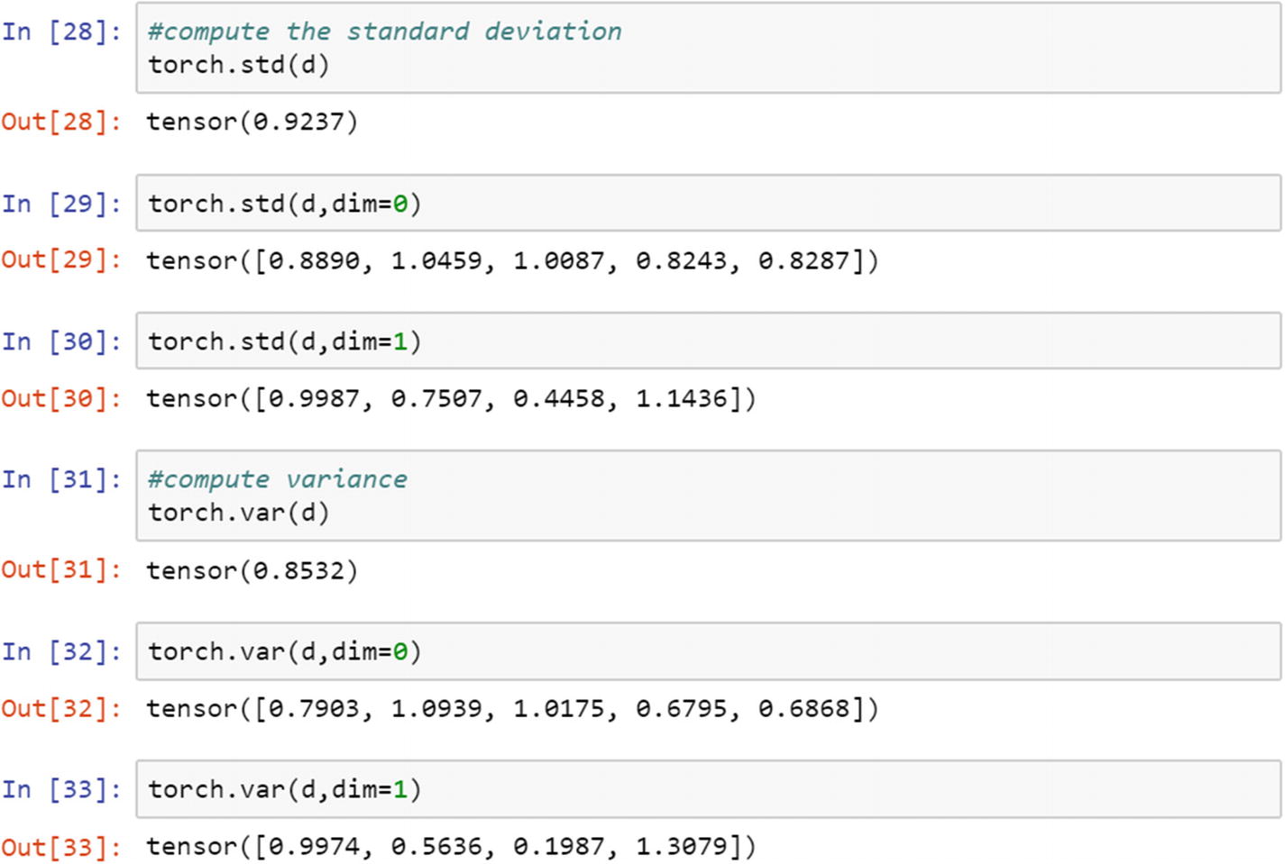
Standard deviation shows the deviation from the measures of central tendency, which indicates the consistency of the data/variable. It shows whether there is enough fluctuation in data or not.
Recipe 2-4. Gradient Computation
Problem
How do we compute basic gradients from the sample tensors using PyTorch?
Solution
We are going to consider a sample datase0074, where two variables (x and y) are present. With the initial weight given, can we computationally get the gradients after each iteration? Let’s take a look at the example.
How It Works
x_data and y_data both are lists. To compute the gradient of the two data lists requires computation of a loss function, a forward pass, and running the stuff in a loop.
The forward function computes the matrix multiplication of the weight tensor with the input tensor.


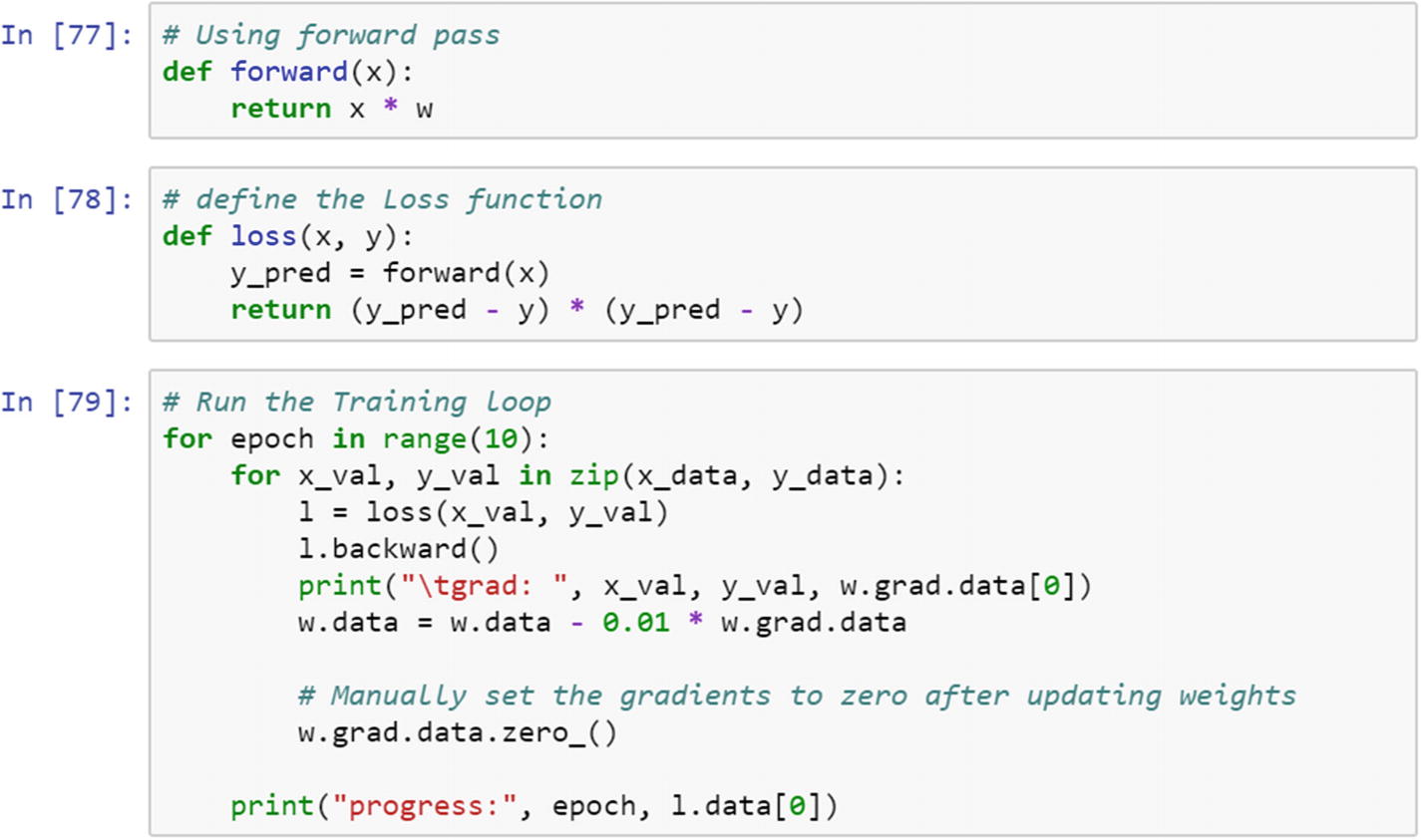
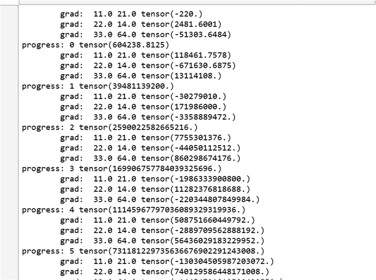

The following program shows how to compute the gradients from a loss function using the variable method on the tensor.
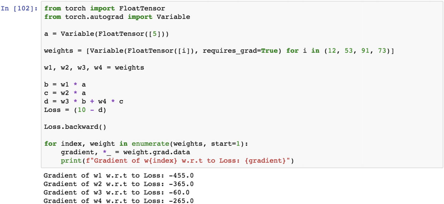
Recipe 2-5. Tensor Operations
Problem
How do we compute or perform operations based on variables such as matrix multiplication?
Solution
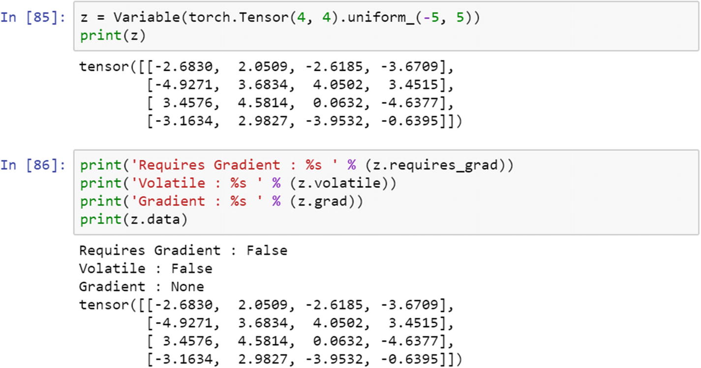
Tensors are wrapped within the variable, which has three properties: grad, volatile, and gradient.
How It Works
Let’s create a variable and extract the properties of the variable. This is required to weight update process requires gradient computation. By using the mm module, we can perform matrix multiplication.

The following program shows the properties of the variable, which is a wrapper around the tensor.
Recipe 2-6. Tensor Operations
Problem
How do we compute or perform operations based on variables such as matrix-vector computation, and matrix-matrix and vector-vector calculation?
Solution
One of the necessary conditions for the success of matrix-based operations is that the length of the tensor needs to match or be compatible for the execution of algebraic expressions.
How It Works
The tensor definition of a scalar is just one number. A 1D tensor is a vector, and a 2D tensor is a matrix. When it extends to an n dimensional level, it can be generalized to only tensors. When performing algebraic computations in PyTorch, the dimension of a matrix and a vector or scalar should be compatible.


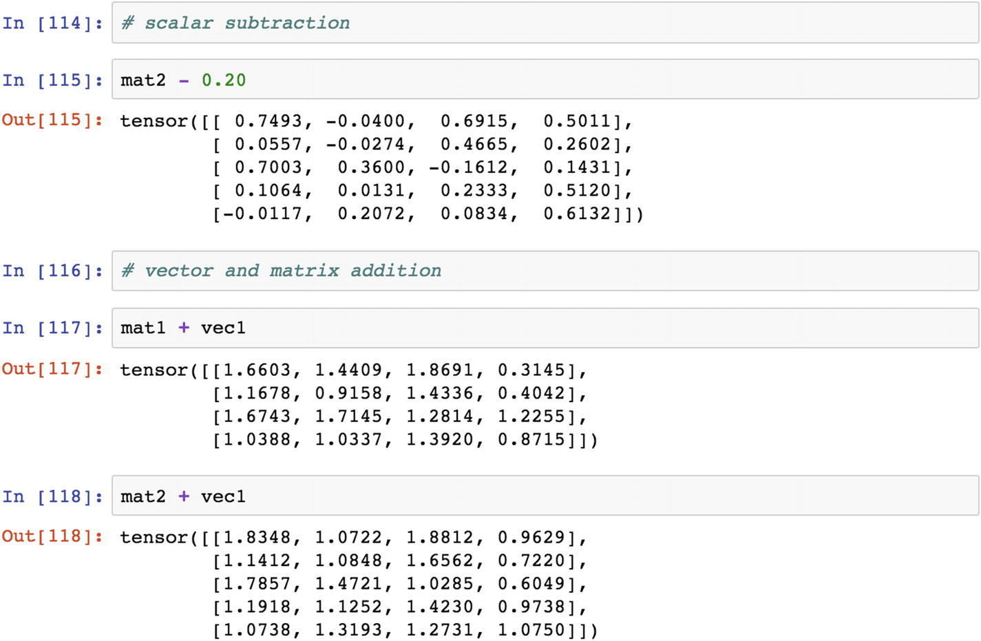
Since the mat1 and the mat2 dimensions are different, they are not compatible for matrix addition or multiplication. If the dimension remains the same, we can multiply them. In the following script, the matrix addition throws an error when we multiply similar dimensions—mat1 with mat1. We get relevant results.


Recipe 2-7. Distributions
Problem
Knowledge of statistical distributions is essential for weight normalization, weight initialization, and computation of gradients in neural network–based operations using PyTorch. How do we know which distributions to use and when to use them?
Solution
Each statistical distribution follows a pre-established mathematical formula. We are going to use the most commonly used statistical distributions, their arguments in scenarios of problems.
How It Works
Bernoulli distribution is a special case of binomial distribution , in which the number of trials can be more than one; but in a Bernoulli distribution, the number of experiment or trial remains one. It is a discrete probability distribution of a random variable, which takes a value of 1 when there is probability that an event is a success, and takes a value of 0 when there is probability that an event is a failure. A perfect example of this is tossing a coin, where 1 is heads and 0 is tails. Let’s look at the program.
The beta distribution is a family of continuous random variables defined in the range of 0 and 1. This distribution is typically used for Bayesian inference analysis.

The binomial distribution is applicable when the outcome is twofold and the experiment is repetitive. It belongs to the family of discrete probability distribution, where the probability of success is defined as 1 and the probability of failure is 0. The binomial distribution is used to model the number of successful events over many trials.

In probability and statistics, a categorical distribution can be defined as a generalized Bernoulli distribution, which is a discrete probability distribution that explains the possible results of any random variable that may take on one of the possible categories, with the probability of each category exclusively specified in the tensor.

A Laplacian distribution is a continuous probability distribution function that is otherwise known as a double exponential distribution . A Laplacian distribution is used in speech recognition systems to understand prior probabilities. It is also useful in Bayesian regression for deciding prior probabilities.

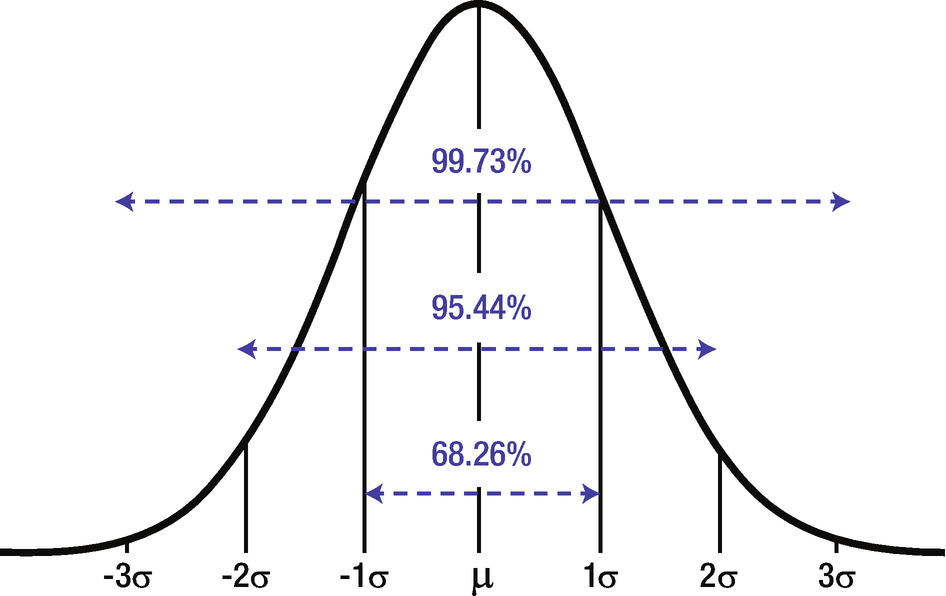
Normal probability distribution

Conclusion
This chapter discussed sampling distribution and generating random numbers from distributions. Neural networks are the primary focus in tensor-based operations. Any sort of machine learning or deep learning model implementation requires gradient computation, updating weight, computing bias, and continuously updating the bias.
This chapter also discussed the statistical distributions supported by PyTorch and the situations where each type of distribution can be applied.
The next chapter discusses deep learning models in detail. Those deep learning models include convolutional neural networks, recurrent neural networks, deep neural networks, and autoencoder models.