measure and a root MSE difference statistic.
Chapter 8
Statistical and Economic Methods for Evaluating Exchange Rate Predictability
Exchange rate fluctuations are regularly monitored with great interest by policy makers, practitioners, and academics. It is not surprising, therefore, that exchange rate predictability has long been at the top of the research agenda in international finance. Starting with the seminal contribution of Meese and Rogoff (1983), a large body of empirical research finds that models that depend on economically meaningful variables do not provide reliable exchange rate forecasts. This has led to the prevailing view that exchange rates follow a random walk (RW) and hence are not predictable, especially at short horizons.
Several well-known puzzles in foreign exchange (FX) are responsible for this view. First, the “exchange rate disconnect puzzle” concerns the empirical disconnect between exchange rate movements and economic fundamentals such as money supply and real output (Cheung et al., 2005; Mark, 1995; Rogoff and Stavrakeva, 2008). Second, the “forward premium puzzle” implies that on average the interest differential is not offset by a commensurate depreciation of the investment currency, which is an empirical violation of uncovered interest rate parity. As a result, borrowing in low interest rate currencies and investing in high interest rate currencies forms the basis of the widely used carry trade strategy in active currency management (Brunnermeier et al., 2009; Burnside et al., 2011; Fama, 1984; and Della Corte et al., 2009). Third, there is extensive evidence that purchasing power parity (PPP) holds in the long run (Lothian and Taylor, 1996).
A recent contribution by Engel and West (2005) provides a possible resolution to the difficulty of tying exchange rates to economic fundamentals. Specifically, Engel and West (2005) show analytically that exchange rates can be consistent with present value asset pricing models and still manifest near-RW behavior if two conditions are met: (i) fundamentals integrated are of order 1 and (ii) the discount factor for future fundamentals is near 1.1
A model that is nested by the Engel and West (2005) present value relation is a variant of the Taylor (1993) rule used for exchange rate determination. The Taylor rule postulates that the central bank adjusts the short-run nominal interest rate in response to changes in inflation, the output gap, and the exchange rate. Using alternative specifications of Taylor rule fundamentals, Molodtsova and Papell (2009) provide strong evidence of short-horizon exchange rate predictability and hence offer renewed hope for empirical success in this literature. In short, one way to summarize the state of the literature is that it has come full circle: from the Meese and Rogoff (1983) “no predictability at short horizons,” to the Mark (1995) “predictability at long but not at short horizons,” to the Cheung et al. (2005) “no predictability at any horizon,” to finally, the Molodtsova and Papell (2009) “predictability at short horizons with Taylor rule fundamentals.”
This chapter aims at connecting these related literatures by providing a comprehensive review of the statistical and economic methods used for evaluating exchange rate predictability, especially out of sample. We assess the short-horizon forecasting performance of a set of widely used empirical exchange rate models that include the RW model, uncovered interest parity, PPP, monetary fundamentals (MF), and TRs and TRa. Our analysis employs monthly FX data ranging from January 1976 to June 2010 for the 10 most liquid (G10) currencies in the world: the Australian dollar (AUD), Canadian dollar (CAD), Swiss franc (CHF), Deutsche mark \ euro (EUR), British pound (GBP), Japanese yen (JPY), Norwegian kroner (NOK), New Zealand dollar (NZD), Swedish kronor (SEK), and US dollar (USD).2
The vast majority of the FX literature uses a well-established statistical methodology for evaluating exchange rate predictability. This methodology typically involves statistical tests of the null hypothesis of equal predictive ability between the RW benchmark and an alternative empirical exchange rate model. The tests are based on the out-of-sample (OOS) mean squared error (MSE) of the forecasts generated by the models. In this chapter, we discuss the main recent contributions to this methodology.
The most popular method for testing whether the alternative model has a lower MSE than the benchmark is using the Diebold and Mariano (1995) and West (1996) statistic. By design, however, all the models we estimate are nested, and this statistic has a nonstandard distribution when comparing forecasts from nested models. Therefore, we focus on the recent inference procedure by Clark and West (2006, 2007), which accounts for the fact that under the null, the MSE from the alternative model is expected to be greater than that from the RW benchmark because the alternative model introduces noise into the forecasting process by estimating a parameter vector that is not helpful in prediction. For a comprehensive statistical evaluation, we also implement the encompassing test of Clark and McCracken (2001) and the F-statistic of McCracken (2007) using bootstrapped critical values. Finally, following Campbell and Thompson (2008) and Welch and Goyal (2008), we also report the OOS measure and a root MSE difference statistic.
In addition to the extensive literature on statistical evaluation, there is also an emerging line of research proposing a methodology for assessing the economic value of exchange rate predictability. A purely statistical analysis of predictability is not particularly informative to an investor, as it falls short of measuring whether there are tangible economic gains from using dynamic forecasts in active portfolio management. We review this approach on the basis of the dynamic asset allocation that is used, among others, by Abhyankar et al. (2005), Bandi and Russell (2006), Bandi et al. (2008), Della Corte et al. (2008), Fleming et al. (2001), Han (2006), Marquering and Verbeek (2004), West et al. (1993) and Della Corte et al. (2009, 2011).
We first design an international asset allocation strategy that exposes a US investor purely to FX risk. The investor builds a portfolio by allocating her wealth between a domestic and a set of foreign bonds and then uses the exchange rate forecasts from each model to predict the USD return of the foreign bonds. We evaluate the performance of the dynamically rebalanced portfolios using mean-variance analysis, which allows us to measure how much a risk-averse investor is willing to pay for switching from a portfolio strategy based on the RW benchmark to an empirical exchange rate model that conditions on economic fundamentals. In contrast to statistical measures of forecast accuracy that are computed separately for each exchange rate, the economic value is assessed for the portfolio generated by a model's forecasts on all exchange rate returns. This contributes to our finding that even modest statistical significance in OOS predictive regressions can lead to large economic benefits for investors.
Our review also includes an assessment of the economic value of combined forecasts. We use a variety of model averaging methods, some of which generate forecast combinations in a naive ad hoc manner, some that exploit statistical measures of past OOS forecasting performance, and some that use economic measures of past predictability. All forecast combinations that we explore are formed ex-ante using the full universe of individual forecasts of each model for each exchange rate. It is important to note that the combined forecasts do not require a view of which model is best at any given period and therefore provide a way for resolving model uncertainty.
To preview our key results, we find strong statistical and economic evidence against the RW benchmark. In particular, empirical exchange rate models based on uncovered interest parity (UIP), PPP, and the TRa perform better than the RW in OOS prediction using both statistical and economic criteria. We also confirm that conditioning on MF does not generate OOS economic gains. Consistently, the worst performing model is the symmetric Taylor rule (TRs). Finally, combined forecasts formed using a variety of model averaging methods perform even better than individual empirical models. These results are robust to reasonably high transaction costs, the choice of numeraire, and the exclusion of any one currency from the investment opportunity set.
The remainder of the chapter is organized as follows. In the next section, we briefly review the empirical exchange rate models that we estimate and their foundations in asset pricing. Section 8.3 describes the statistical methods we use for evaluating exchange rate predictability. In Section 8.4 we present a general framework for assessing the economic value of forecasting exchange rates for a risk-averse investor with a dynamic mean-variance portfolio allocation strategy. Section 8.5 explains the construction of combined forecasts using a variety of model averaging methods. Section 8.6 reports our empirical results and, finally, Section 8.7 provides the concluding remarks.
In this section, we review the empirical models that we use for evaluating exchange rate predictability. We begin by describing the Engel and West (2005) present value model that nests and motivates many of the predictive regressions we estimate.
The Engel and West (2005) model relates the exchange rate to economic fundamentals and the expected future exchange rate as follows:
8.1 
where st is the log of the nominal exchange rate defined as the domestic price of foreign currency, fi, t (i = 1, 2) are the observed economic fundamentals, and zi, t are the unobserved fundamentals that drive the exchange rate. Note that an increase in st implies a depreciation of the domestic currency. This is a general asset pricing model that builds on earlier work on pricing stock returns by Campbell and Shiller (1987, 1988) and West (1988).
Iterating forward and imposing the no-bubbles condition leads to the following present value relation:
8.2 
Engel and West (2005) show that the exchange rate will follow a RW if the discount factor b is close to 1 and either (i)  and f2, t + z2, t = 0 or (ii)
  . Some other well-known exchange rate models take the general form of Equation (1), and in what follows, we discuss two examples.
Consider first the monetary exchange rate models of the 1970s and 1980s, which assume that the money market relation is described by
where mt is the log of the domestic money supply, pt is the log of the domestic price level, γ > 0 is the income elasticity of money demand, yt is the log of the domestic national income, α > 0 is the interest rate semielasticity of money demand, it is the domestic nominal interest rate, and vm, t is a shock to domestic money demand. A similar equation holds for the foreign economy, where the corresponding variables are denoted by  ,
,  ,
,  ,
,  , and
, and  . We assume that the parameters
  of the foreign money demand are identical to the domestic parameters.
The nominal exchange rate is equal to its PPP value plus the real exchange rate qt
8.4 
Finally, the interest parity condition is given by
8.5 
where ρt is the deviation from the UIP condition that is based on rational expectations and risk neutrality. Hence ρt can be interpreted either as an expectational error or a risk premium.
Using Equations (8.3)–(8.5) for the domestic and foreign economies and rearranging, we get
8.6 
This equation takes the form of the original model in Equation (8.1), where the discount factor is given by b = α/1 + α, the observable fundamentals are  , and the unobservable fundamentals are
  and z2, t = − ρt.
The second model to be nested by the Engel and West (2005) present value relation is the Taylor (1993) rule, where the home country is assumed to set the short-term nominal interest rate according to
8.7 
where i is the target short-term interest rate,  is the output gap measured as the percentage deviation of actual real GDP from an estimate of its potential level, πt is the inflation rate,
  is the target inflation rate, and vt is a shock. The Taylor rule postulates that the central bank raises the short-term nominal interest rate when output is above potential output and/or inflation rises above its desired level.
The foreign country is assumed to follow a Taylor rule that explicitly targets exchange rates (Clarida et al., 1998):
8.8 
where 0 < β0 < 1 and st is the target exchange rate. For simplicity, we assume that the home and foreign countries target the same interest rate, i, and the same inflation rate,  . The rule indicates that the foreign country raises interest rates when its currency depreciates relative to the target.3
We assume that the foreign central bank targets the PPP level of the exchange rate
8.9 
Taking the difference between the home and foreign Taylor rules, using interest parity (Eq. 8.5), substituting the target exchange rate, and solving for st gives
8.10 
This equation also has the general form of the present value model in Equation (Eq. 8.1), where the discount factor is b = 1/1 + β0,  and
and  .
.
Our empirical analysis is based on six predictive regressions for exchange rate returns, many of which are nested and motivated by the Engel and West (2005) present value model. All predictive regressions have the following same linear structure:
8.11 
where Δst+1 = st+1 − st, α and β are constants to be estimated, and ε t+1 is a normal error term. The empirical models differ in the way they specify the economic fundamentals xt that are used to forecast exchange rate returns.
The first regression is the RW with drift model that sets β = 0. Since the seminal work of Meese and Rogoff (1983), this model has become the benchmark in assessing exchange rate predictability. The RW model captures the prevailing view in international finance research that exchange rates are not predictable when conditioning on economic fundamentals, especially at short horizons.
The second regression is based on the UIP condition:4
8.12 
UIP is the cornerstone condition for FX market efficiency. Assuming risk neutrality and rational expectations, it implies that α = 0, β = 1, and the error term is serially uncorrelated. However, numerous empirical studies consistently reject the UIP condition (Engel, 1996; Hodrick, 1987; Sarno, 2005). As a result, it is a stylized fact that estimates of β tend to be closer to minus unity than plus unity. This is commonly referred to as the “forward premium puzzle,” which implies that high interest currencies tend to appreciate rather than depreciate and forms the basis of the widely used carry trade strategy in active currency management.5
The third regression is based on the PPP hypothesis
8.13 
The PPP hypothesis states that national price levels should be equal when expressed in a common currency and is typically thought of as a long-run condition rather than holding at each point in time (Rogoff, 1996; Taylor and Taylor, 2004).
The fourth regression conditions on MF:
The relation between exchange rates and fundamentals defined in Equation (8.14) suggests that a deviation of the nominal exchange rate st+1 from its long-run equilibrium level determined by the fundamentals xt, requires the exchange rate to move in the future so as to converge toward its long-run equilibrium. The empirical evidence on the relation between exchange rates and fundamentals is mixed. On the one hand, short-run exchange rate variability appears to be disconnected from the underlying fundamentals (Mark, 1995) in what is commonly referred to as the “exchange rate disconnect puzzle.” On the other hand, some recent empirical research finds that fundamentals and nominal exchange rates move together in the long run (Groen, 2000; Mark and Sul, 2001).
The final two regressions are based on simple versions of the Taylor (1993) rule. We estimate a TRs
8.15 
as well as an TRa that assumes that the foreign central bank also targets the real exchange rate
8.16 
The domestic and foreign output gaps are computed with a Hodrick and Prescott (1997) (HP) filter.6 The parameters on the inflation difference (1.5), output gap difference (0.1), and the real exchange rate (0.1) are fairly standard in the literature (Engel et al., 2007; Mark, 2009). Alternative versions of the Taylor rule that we do not consider in this chapter may also account for smoothing, where interest rate adjustments are not immediate but gradual, and heterogeneous coefficients for (i) the US versus foreign inflation and (ii) the US versus foreign output gap (Molodtsova and Papell, 2009).
The success or failure of empirical exchange rate models is typically determined by statistical tests of OOS predictive ability. Our statistical analysis tests for equal predictive ability between one of the empirical exchange rate models we estimate (UIP, PPP, MF, TRs, or TRa) and the benchmark RW model. In effect, we are comparing the performance of a parsimonious restricted null model (the RW, where β = 0) to a set of larger alternative unrestricted models that nest the parsimonious model (where  ).7
).7
We estimate all empirical exchange rate models using ordinary least squares (OLS) and then run a pseudo-OOS forecasting exercise as follows (Stock and Watson, 2003). Given today's known observables  , we define an in-sample (IS) period using observations
  , and an OOS period using
  . This exercise produces
  OOS forecasts. Our empirical analysis uses T − 1 = 413 monthly observations, M = 120, and P = 293.8
In what follows, we describe a comprehensive set of statistical criteria for evaluating the OOS predictive ability of empirical exchange rate models. First, we compute the Campbell and Thompson (2008) OOS R2 statistic,  , that compares the unconditional forecasts of the benchmark RW model to the conditional forecasts of an alternative model. Let Δst+1|t denote the one-step-ahead unconditional forecast from the RW and
  be the one-step-ahead conditional forecast from the alternative model represented by one of Equations (8.12)–(8.16). Then, the
  statistic is given by
A positive  statistic implies that the alternative model outperforms the benchmark RW by having a lower MSE.
Second, we compute the OOS root MSE difference statistic, ΔRMSE, as in Welch and Goyal (2008).

A positive ΔRMSE denotes that the alternative model outperforms the benchmark RW by having a lower RMSE.
The most popular method for testing whether the alternative model has a lower MSE than the benchmark is using the Diebold and Mariano (1995) and West (1996) statistic, which has an asymptotic standard normal distribution when comparing forecasts from nonnested models. However, as shown by Clark and McCracken (2001) and McCracken (2007), this statistic has a nonstandard distribution when comparing forecasts from nested models and is severely undersized when using standard normal critical values. Clark and McCracken (2001) and McCracken (2007) account for this size distortion by deriving the nonstandard asymptotic distributions for a number of statistical tests as applied to nested models. We report the two tests with the best overall power and size properties: the ENC-F encompassing test statistic proposed by Clark and McCracken (2001) defined as follows:

and the MSE-F test of McCracken (2007):
When the models are correctly specified, the forecast errors are serially uncorrelated and exhibit conditional homoskedasticity. In this case, Clark and McCracken (2001) and McCracken (2007) numerically generated the asymptotic critical values for the ENC-F and MSE-F tests. When the above conditions are not satisfied, a bootstrap procedure must be used to compute valid critical values, which we discuss later.
Finally, we also apply the recently developed inference procedure by Clark and West (2006, 2007) for testing the null of equal predictive ability of two nested models. This procedure acknowledges the fact that under the null the MSE from the alternative model is expected to be greater than that of the RW benchmark because the alternative model introduces noise into the forecasting process by estimating a parameter vector that is not helpful in prediction. Therefore, finding that the RW has smaller MSE is not clear evidence against the alternative model. Clark and West (2006, 2007) suggest that the MSE should be adjusted as follows:
8.17 
Then, a computationally convenient way of testing for equal MSE is to define
8.18 
and to regress  on a constant, using the t-statistic for a zero coefficient, which we denote by MSE-t. Even though the asymptotic distribution of this test is nonstandard (Clark and West (2006, 2007); McCracken, 2007) show that standard normal critical values provide a good approximation and therefore recommend to reject the null if the statistic is greater than + 1.282 (for a one-sided 0.10 test) or + 1.645 (for a one-sided 0.05 test).9
The above statistical tests compare the null hypothesis of equal forecast accuracy with the one-sided alternative that forecasts from the unrestricted model are more accurate than those from the restricted benchmark model. Asymptotic critical values for these test statistics, whenever available, tend to be severely biased in small samples. In addition to the size distortion, there may be spurious evidence of return predictability in small samples when the forecasting variable is sufficiently persistent (Nelson and Kim, 1993; Stambaugh, 1999). In order to address these concerns, we obtain bootstrapped critical values for a one-sided test by estimating the model and generating 10, 000 bootstrapped time series under the null. The procedure preserves the autocorrelation structure of the predictive variable and maintains the cross-correlation structure of the residual. The bootstrap algorithm is summarized in Appendix A.
This section describes the framework for evaluating the performance of an asset allocation strategy that exploits predictability in exchange rate returns.
We design an international asset allocation strategy that involves trading the USD and nine other currencies: the AUD, CAD, CHF, Deutsche mark \ euro (EUR), GBP, JPY, NOK, NZD, and SEK. Consider a US investor who builds a portfolio by allocating her wealth between 10 bonds: one domestic (US), and nine foreign bonds (Australia, Canada, Switzerland, Germany, UK, Japan, Norway, New Zealand, and Sweden). The yield of the bonds is proxied by euro deposit rates. At each period t + 1, the foreign bonds yield a riskless return in local currency but a risky return rt+1 in USD, whose expectation at time t is equal to Et[rt+1] = it + Δst+1|t. Hence the only risk the US investor is exposed to is the FX risk.
In each period the investor takes two steps. First, she uses each predictive regression to forecast the one-period-ahead exchange rate returns. Second, depending on the forecasts of each model, she dynamically rebalances her portfolio by computing the new optimal weights. This setup is designed to assess the economic value of exchange rate predictability by informing us which empirical exchange rate model leads to a better performing allocation strategy.
Mean-variance analysis is a natural framework for assessing the economic value of strategies that exploit predictability in the mean and variance. Consider an investor who has a one-period horizon and constructs a dynamically rebalanced portfolio. Computing the time-varying weights of this portfolio requires one-step-ahead forecasts of the conditional mean and the conditional variance–covariance matrix. Let rt+1 denote the  vector of risky asset returns; μt+1|t = Et[rt+1] is the conditional expectation of rt+1 and Σt+1|t = Et[(rt+1 − μt+1|t)(rt+1 − μt+1|t)′] is the K × K conditional variance–covariance matrix of rt+1.
Mean-variance analysis may involve three rules for optimal asset allocation: maximum expected utility, maximum expected return, and minimum volatility. Following Della Corte et al. (2009, 2011), our empirical analysis focuses on the maximum expected return strategy, as this is the strategy most often used in active currency management. For details on the maximum expected utility rule and the minimum volatility rule see Han (2006).
The maximum expected return rule leads to a portfolio allocation on the efficient frontier for a given target conditional volatility. At each period t, the investor solves the following problem:
8.19 
8.20 
where  is the target conditional volatility of the portfolio returns. The solution to the maximum expected return rule gives the following risky asset weights:
8.21 
where 
Then, the gross return on the investor's portfolio is
8.22 
Note that we assume that  , where
  is the unconditional covariance matrix of exchange rates returns using available information at time t. In other words, we do not model the dynamics of FX return volatility and correlation. Therefore, the optimal weights will vary across the empirical exchange rate models only to the extent that the predictive regressions produce better forecasts of the exchange rate returns.10
We assess the economic value of exchange rate predictability with a set of standard mean-variance performance measures. We begin our discussion with the Fleming et al. (2001) performance fee, which is based on the principle that at any point in time, one set of forecasts is better than another if investment decisions based on the first set lead to higher average realized utility. The performance fee is computed by equating the average utility of the RW optimal portfolio with the average utility of the alternative (e.g., UIP) optimal portfolio, where the latter is subject to expenses  . Since the investor is indifferent to these two strategies, we interpret
  as the maximum performance fee she will pay to switch from the RW to the alternative (e.g., UIP) strategy. In other words, this utility-based criterion measures how much a mean-variance investor is willing to pay for conditioning on better exchange rate forecasts. The performance fee will depend on δ, which is the investor's degree of relative risk aversion (RRA). To estimate the fee, we find the value of
  that satisfies
8.23 
where  is the gross portfolio return constructed using the forecasts from the alternative (e.g., UIP) model and Rp, t+1 is the gross portfolio return implied by the benchmark RW model.
We also evaluate performance using the premium return, which builds on the Goetzmann et al. (2007) manipulation-proof performance measure and is defined as
8.24 
where Rf = 1 + rf.  is robust to the distribution of portfolio returns and does not require the assumption of a particular utility function to rank portfolios. In contrast, the Fleming et al. (2001) performance fee assumes a quadratic utility function.
  can be interpreted as the certainty equivalent of the excess portfolio returns and hence can also be viewed as the maximum performance fee an investor will pay to switch from the benchmark to another strategy. In other words, this criterion measures the risk-adjusted excess return an investor enjoys for using one particular exchange rate model rather than assuming a RW. We report both
  and
and  in annualized basis points (bps).
In the context of mean-variance analysis, perhaps the most commonly used measure of economic value is the Sharpe ratio ( ). The realized
  is equal to the average excess return of a portfolio divided by the standard deviation of the portfolio returns. It is well known that because the
  uses the sample standard deviation of the realized portfolio returns, it overestimates the conditional risk an investor faces at each point in time and hence underestimates the performance of dynamic strategies (Han, 2006; Marquering and Verbeek, 2004).
Finally, we also compute the Sortino ratio ( ), which measures the excess return to “bad” volatility. Unlike the
  , the
, the  differentiates between volatility due to “up” and “down” movements in portfolio returns. It is equal to the average excess return divided by the standard deviation of only the negative returns. In other words, the
  does not take into account positive returns in computing volatility because these are desirable. A large
  indicates a low risk of large losses.
The effect of transaction costs is an essential consideration in assessing the profitability of dynamic trading strategies. We account for this effect in three ways. First, we calculate the performance measures for the case when the bid-ask spread for spot exchange rates is equal to 8 bps. In foreign exchange trading, this is a realistic range for the recent level of transaction costs.11 We follow the simple approximation of Marquering and Verbeek (2004) by deducting the proportional transaction cost from the portfolio return ex-post. This ignores the fact that dynamic portfolios are no longer optimal in the presence of transaction costs but maintain simplicity and tractability in our analysis.12
The second way of accounting for transaction costs acknowledges the fact that for long data samples the transaction costs will likely change over time. Neely et al. (2009) find that the transaction cost for switching from a long to a short position in FX has on an average declined from about 10 bps in the 1970s to about 2 bps in recent years. If we were to keep transaction costs constant over our sample period, we would spuriously introduce a decline in performance by penalizing more recent returns too heavily relative to those early in the sample period. Therefore, we follow Neely et al. (2009) in estimating a simple time trend that assumes that the bid-ask spread was 20 bps at the beginning of our data sample and declined linearly to 4 bps by the end of the sample. The actual one-way transaction cost is half of the bid-ask spread and hence declines from 10 bps to 2 bps. Specifically, the net return from buying a currency at the spot exchange rate at time t and selling at time t + 1 is equal to  , where
  and
and  is the one-way transaction cost (Neely et al. 2009). St is the spot exchange rate and st is st = lnSt. In the first case, we assume a fixed bid-ask spread and hence τt = τ, whereas in the second case, τt is time-varying.13
Third, we also calculate the break-even proportional transaction cost, τbe, that renders investors indifferent to two strategies (Han, 2006). We assume that τ is a fixed fraction of the value traded in all assets in the portfolio. Then, the cost of the dynamic strategy is  for each asset j ≤ K. In comparing a dynamic strategy with the benchmark RW strategy, an investor who pays transaction costs lower than τbe will prefer the dynamic strategy. Since τbe is the proportional cost paid every time the portfolio is rebalanced, we report τbe in monthly basis points.14
Our analysis has so far focused on evaluating the performance of individual empirical exchange rate models relative to the RW benchmark. Considering a large set of alternative models that capture different aspects of exchange rate behavior without knowing which model is “true” (or best) inevitably generates model uncertainty. In this section, we resolve this uncertainty by exploring whether portfolio performance improves when combining the forecasts arising from the full set of predictive regressions. Even though the potentially superior performance of combined forecasts is known since the seminal work of Bates and Granger (1969), applications in finance are only recently becoming increasingly popular (Timmermann, 2006). Rapach et al. (2010) argue that forecast combinations can deliver statistically and economically significant OOS gains for two reasons: (i) they reduce forecast volatility relative to individual forecasts and (ii) they are linked to the real economy.15
Recall that we estimate N = 6 predictive regressions, each of which provides an individual forecast  for the one-step-ahead exchange rate return, where i ≤ N. We define the combined forecast
  as the weighted average of the N individual forecasts
  :
:
8.25 
where  are the ex-ante combining weights determined at time t.
We form three types of combined forecasts. The first one uses simple model averaging that, in turn, implements three rules: (i) the mean of the panel of forecasts so that ωi, t = 1/N; (ii) the median of the  individual forecasts; and (iii) the trimmed mean that sets ωi, t = 0 for the individual forecasts with the smallest and largest values and
  for the remaining individual forecasts. These combined forecasts disregard the historical performance of the individual forecasts.
The second type of combined forecasts is based on Stock and Watson (2004) and uses statistical information on the past OOS performance of each individual model. In particular, we compute the discounted MSE (DMSE) forecast combination by setting the following weights:
8.26 
where θ is a discount factor and M are the first IS observations on which we depend to form the first OOS forecast. For θ < 1, greater weight is attached to the most recent forecast accuracy of the individual models. The DMSE forecasts are computed for three values of θ = {0.90, 0.95, 1.0}. The case of no discounting (θ = 1) corresponds to the Bates and Granger (1969) optimal forecast combination when the individual forecasts are uncorrelated. We also compute simpler “most recently best” MSE(κ) forecast combinations that use no discounting (θ = 1) and weigh individual forecasts by the inverse of the OOS MSE computed over the last κ months, where κ = {12, 36, 60}.
The third type of combined forecasts does not use statistical information on the historical performance of individual forecasts. Instead it exploits the economic information contained in the Sharpe ratio ( ) of the portfolio returns generated by an individual forecasting model over a prespecified recent period. We compute the discounted
  (DSR) combined forecast by setting the following weights:
8.27 
Finally, we also compute simpler “most recently best”  forecast combinations that use no discounting (θ = 1) and weigh individual forecasts by the OOS
  computed over the last κ months, where
  .
.
We assess the economic value of combined forecasts by treating them in the same way as any of the individual empirical models. For instance, we compute the performance fee,  , for the DMSE one-month-ahead forecasts and compare it to the RW benchmark. Finally, note that where possible, we use these forecast combination methods not only for the OOS mean prediction but also for the OOS variance covariance matrix that enters the weights in mean-variance asset allocation.
The data sample consists of 414 monthly observations ranging from January 1976 to June 2010 and focuses on nine spot exchange rates relative to the USD: the AUD, CAD, CHF, Deutsche mark \ euro (EUR), GBP, JPY, NOK, NZD, and SEK. The exchange rate is defined as the USD price of a unit of foreign currency so that an increase in the exchange rate implies a depreciation of the USD. These data are obtained through the download data program (DDP) of the Board of Governors of the Federal Reserve System.16
Table 8.1 provides a detailed description of all data sources we use. For interest rates, we use the one-month euro deposit rate taken from Datastream with the following exceptions. For Japan, the euro deposit rate is only available from January 1979, and hence before this date, we use CIP relative to the USD to construct the no-arbitrage riskless rate. The one-month forward exchange rate required to implement CIP is taken from Hai et al. (1997). For Australia, Norway, New Zealand, and Sweden, euro deposit rates are only available from April 1997. For Australia and New Zealand, we combine the money market rate from January 1976 to November 1984 taken from the IMF's International Financial Statistics (IFS) and CIP relative to the USD from December 1984 to March 1997 using one-month forward exchange rates taken from Datastream. For Norway and Sweden, we use CIP relative to GBP from January 1976 to March 1997, using spot and one-month forward exchange rates from Datastream.
Table 8.1 Data Sources

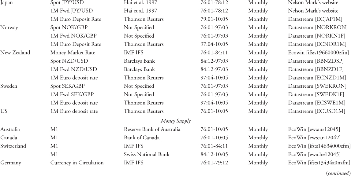
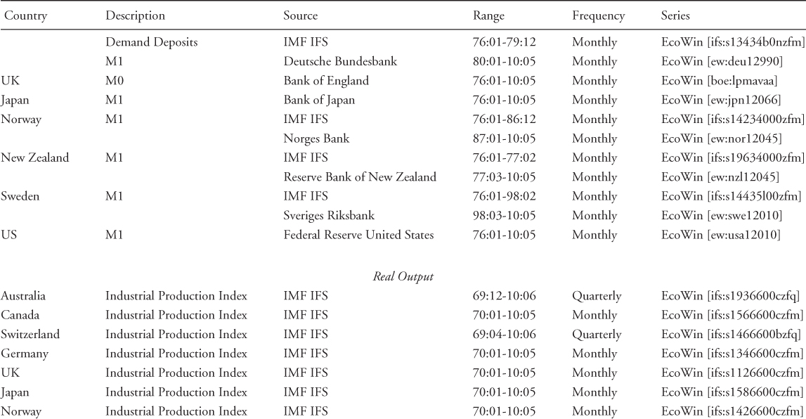
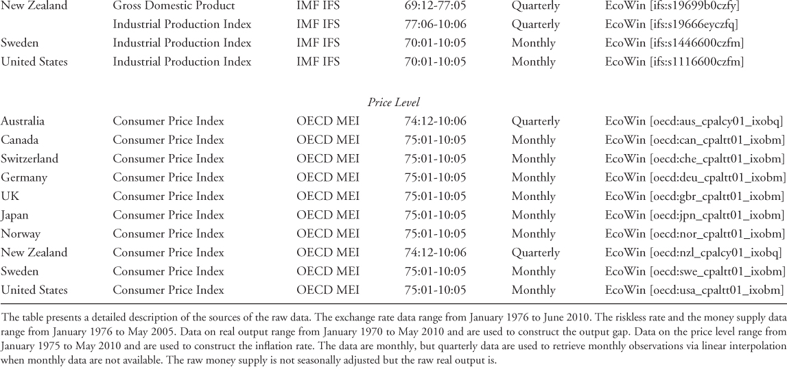
Turning to macroeconomic data, we use nonseasonally adjusted M1 data to measure money supply. For the UK, we use M0 because of the unavailability of M1 data. To construct these times series, we combine IFS and national central bank data from Ecowin.17 We deseasonalize the money supply data by implementing the procedure of Gomez and Maravall (2000).
The price level is measured by the monthly consumer price index (CPI) obtained from the OECD's Main Economic Indicators (MEI). For Australia and New Zealand, CPI data are published at quarterly frequency, and hence monthly observations are constructed by linear interpolation. For the inflation rate, we use an annual measure computed as the 12-month log-difference of the CPI. We define the output gap as deviations from the HP filter.
Since GDP data are generally available quarterly, we proxy real output by the seasonally adjusted monthly industrial production index (IPI) taken from IFS. For Australia, New Zealand, and Switzerland, however, IPI data are only released at quarterly frequency, and hence we obtain monthly observations via
linear interpolation.18 Orphanides (2001) has recently stressed the importance of using real-time data to estimate Taylor rules for the United States, which are data available to central banks when the policy decisions are made. Since real-time data are not available for most of the countries included in this study, we mimic as closely as possible the information set available to the central banks using quasi-real-time data: although data incorporate revisions, we update the HP trend each period so that ex-post data is not used to construct the output gap. In other words, at time t, we only use data up to t − 1 to construct the output gap. Using a number of detrending methods, Orphanides and van Norden (2002) showed that most of the difference between fully revised and real-time data comes from using ex-post data to construct potential output and not from the data revisions themselves.19
We convert all data but interest rates by taking logs and multiplying by 100. Throughout the rest of the chapter, the symbols st, it, mt, pt, πt, yt, and  refer to transformed spot exchange rate, interest rate, money supply, price level, inflation rate, real output, and output gap, respectively. We use an asterisk to denote the transformed data (
 ,
,  ,
,  ,
,  ,
,  , and
, and  ) for the foreign country.
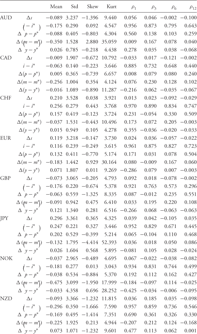
Table 8.2 reports the descriptive statistics for the monthly percentage FX returns, Δst; the difference between domestic and foreign interest rates,  ; the difference in percentage change in price levels,
  ; the difference in percentage change in money supply,
  ; and the difference in percentage change in real output,
  . For our sample period, the monthly sample means of the FX returns range from − 0.138% for SEK to 0.296% for JPY. The return standard deviations are similar across all exchange rates at about 3% per month. Most FX returns exhibit negative skewness and higher-than-normal kurtosis. Finally, the exchange rate return sample autocorrelations are no higher than 0.10 and decay rapidly. For the economic fundamentals, the notable trends are as follows: (i)
  are highly persistent with long memory, (ii)
  are always negatively skewed, and (iii)
  and
and  have occasionally high kurtosis.
Table 8.2 Descriptive Statistics
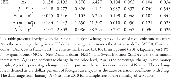
We test the empirical performance of the models by first estimating the six predictive regressions for nine monthly exchange rates. The regressions include the RW model, UIP, PPP, MF, TRs, and TRa. Table 8.3 presents the OLS estimates with Newey and West (1987) standard errors. We focus primarily on the significance of the slope estimate β of the predictive regressions since this would be an indication that the RW benchmark is misspecified.
Table 8.3 Predictive Regressions
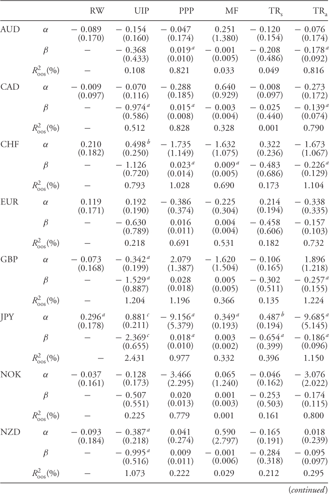
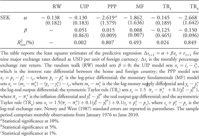
Consistent with the large literature on the forward premium puzzle, the UIP β is predominantly negative. The PPP β is always positive, and for TRa, it is always negative. For these three cases (UIP, PPP and TRa), the β estimates are significant for half of the exchange rates. The least significant slopes are for MF revolving around zero and for TRs for which they are always negative. Finally, the  of the predictive regressions is as high as 2.4%, but in most cases, it is below 1%. In conclusion, the predictive regression results demonstrate that the empirical exchange rates models with the most significant slopes are the UIP, PPP, and TRa.
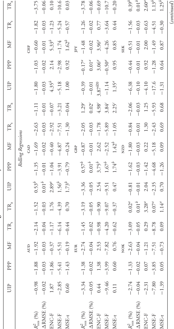
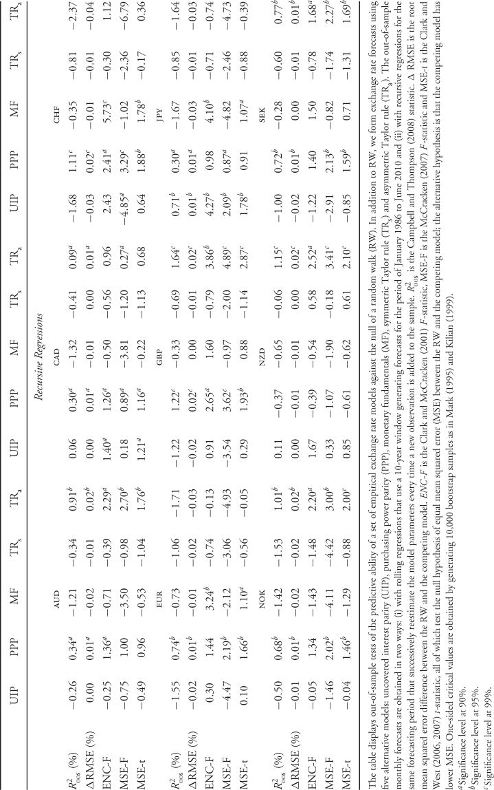
We assess the statistical performance of the empirical exchange rate models (UIP, PPP, MF, TRs, and TRa) by reporting OOS tests of predictability against the null of the RW. We focus on the following statistics:
 statistic of Campbell and Thompson (2008). Recall that a positive
  value implies that the alternative model has lower MSE than the benchmark RW. However, even a slightly negative
  may be consistent with a better performing alternative because the calculation of the
  does take into account the adjustment in the MSE proposed by Clark and West (2006, 2007) to account for the noise introduced in forecasting by estimating a parameter that is not helpful in prediction.
 .
.One-sided critical values are obtained by generating 10,000 bootstrapped time series as in Mark (1995) and Kilian (1999). The OOS monthly forecasts are obtained in two ways: (i) with rolling regressions that use a 10-year window that generates forecasts for the period of January 1986 to June 2010 and (ii) with recursive regressions for the same forecasting period that successively reestimate the model parameters every time a new observation is added to the sample.
Table 8.4 shows that most of the statistics tend to be negative and hence provide evidence against the alternative model. In many cases, however, the results are not statistically significant. If instead we focus on the Clark and West (2006, 2007) MSE-t statistic, which makes the adjustment to the MSE and is hence more reliable, a different picture emerges. For rolling regressions, the UIP and PPP models have a positive MSE-t statistic for seven of the nine exchange rates, whereas the MF and TRa models have for for six. The model that is most often significantly different from the RW is the TRa. The worse performing model is the TRs. The results are very similar for recursive regressions. In short, therefore, a careful examination of the empirical evidence reveals that many of the models perform well against the RW with the clear exception of the TRs.
Table 8.4 Statistical Evaluation of Exchange Rate Predictability
It is important to note that in OOS predictive regressions, lack of statistical significance does not imply lack of economic significance. Campbell and Thompson (2008) show that a small R2 can generate large economic benefits for
investors. They use a mean-variance framework to demonstrate that a good way to judge the magnitude of R2 is to compare it to the square of the Sharpe ratio (SR2). Even a modest R2 can lead to a substantial proportional increase in the expected return by conditioning on the predictive variable xt. Indeed, regressions with large R2 statistics would be too profitable to believe, which is equivalent to the saying “if you are so smart, why aren't you rich?” In the limit, an R2 close to 1 should lead to perfect predictions and hence infinite profits for investors. Furthermore, dynamic asset allocation is, by design, multivariate thus exploiting predictability in all exchange rate series. In the following section, we discuss in detail whether the predictive regressions can generate economic value.
We assess the economic value of exchange rate predictability by analyzing the performance of dynamically rebalanced portfolios based on one-month-ahead forecasts from the six empirical exchange rate models we estimate. The economic evaluation is conducted both IS and OOS, but again, the main focus of our analysis is OOS. The OOS results we present in this section are based on forecasts constructed according to a recursive procedure that only depends on information up to the month in which the forecast is made. The predictive regressions are then successively reestimated every month.
Our empirical analysis focuses on the Sharpe ratio ( ), the Sortino ratio (
 ), the Fleming et al. (2001) performance fee (
 ), the Goetzmann et al. (2007) premium return measure (
 ), and the break-even transaction cost τbe. The
  and
and  performance measures are computed for three cases: (i) zero transaction costs; (ii) a bid-ask spread of 8 bps; and (iii) a bid-ask spread of 20 bps at the beginning of the sample that linearly decays to 4 bps at the end of the sample as suggested by Neely et al. (2009). Following Della Corte et al. (2009, 2011), our empirical analysis focuses on the maximum expected return strategy, as this is the strategy most often used in active currency management. We set a volatility target of
  and a degree of RRA δ = 6. We have experimented with different
  and δ values and found that qualitatively, they have little effect on the asset allocation results discussed below.
Table 8.5 reports the IS and OOS portfolio performance and shows that there is high economic value associated with some of the empirical exchange rate models. We first discuss the IS results, which demonstrate that all models outperform the RW, except for the TRs). For example,  for PPP, 1.28 for TRa, 1.18 for MF, 1.14 for UIP, 1.08 for RW, and 0.96 for TRs. The
  have higher values ranging from 1.26 for TRs to 2.00 for PPP. Switching from the benchmark RW to another model generates
  annual bps for PPP, 202 bps for TRa, 138 for MF, and 83 bps for UIP. The
  performance measure has similar value to
  . Furthermore, both measures are largely unaffected by transaction costs. This can be exemplified by the very large value of the monthly τbe, which are 586 bps for UIP, 328 bps for MF, and 138 bps for PPP.
Table 8.5 The Economic Value of Exchange Rate Predictability
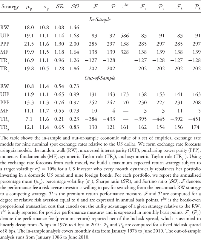
The literature on exchange rate forecasting is primarily concerned with OOS predictability, and hence we turn our attention to the OOS results. The first thing to notice is that the value of the OOS  is smaller than IS. The RW has an OOS
  and is outperformed only by the PPP (
 ), UIP (
 ), and TRa (
 ). Consistent with a very large literature in FX, neither do the MF models outperform the RW nor do the TRs. The
  values are 252 annual bps for PPP, 131 bps for UIP, 130 bps for TRa, 10 bps for MF, and − 384 bps for TRs. The
  measure has slightly higher value than
  . Transaction costs seem to be a bit more important OOS than IS. For example, the τbe are 173 bps for UIP, 161 bps for TRa, and 70 bps for PPP. However, it seems that whether we assume fixed transaction costs or linearly decaying costs makes little difference in the performance of the empirical exchange rate models. In short, our findings demonstrate that it is worth using the UIP, PPP, and TRa empirical exchange rate models, as their forecasts generate significant economic value.
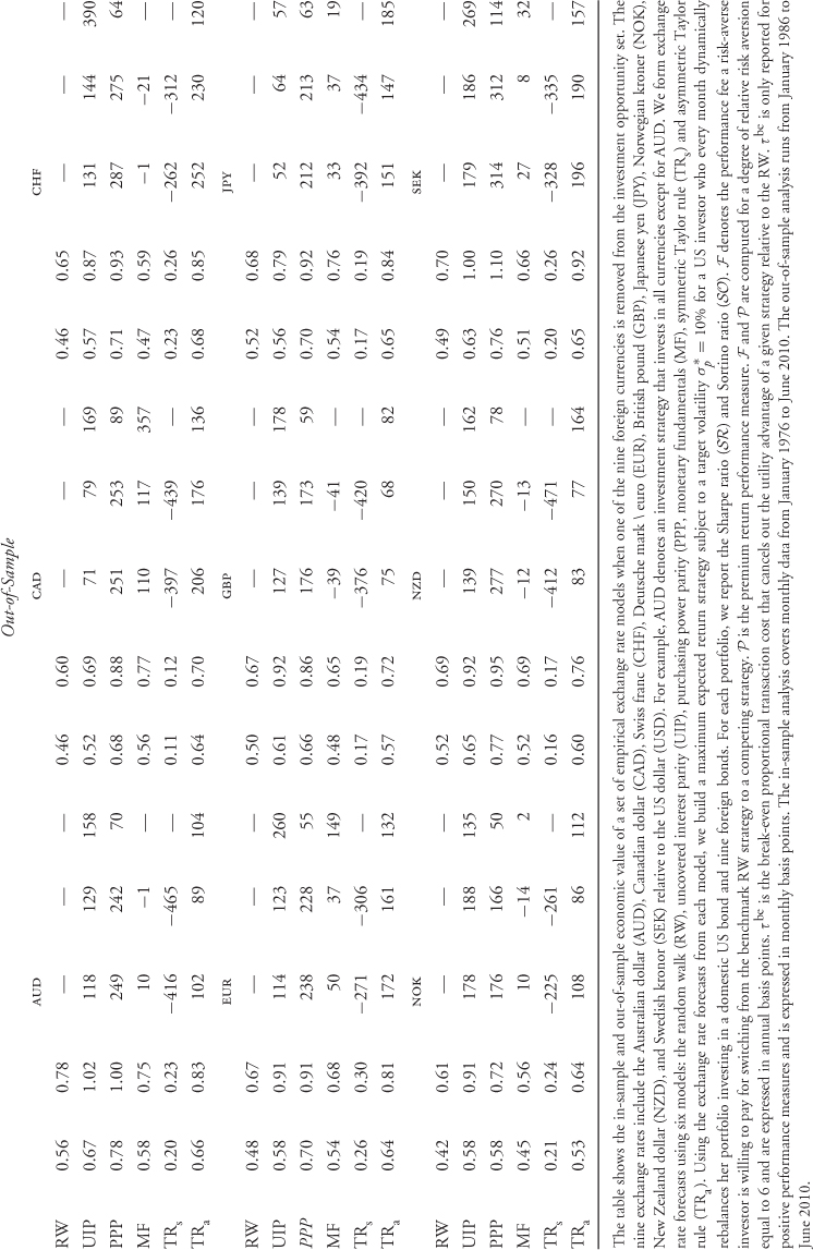
By design, the dynamic FX strategy invests in nine foreign bonds and thus exploits predictability in nine exchange rates. Since we economically evaluate the performance of portfolios rather than individual exchange rates, it would be interesting to assess whether the superior portfolio performance of one versus another empirical model is driven by one particular currency. Table 8.6 reports the economic value of exchange rate predictability when we remove one of the currencies (and hence one of the bonds) from the investment opportunity set. For example, AUD in Table 8.6 denotes the dynamic allocation strategy that invests in all currencies, except for AUD. The results for excluding one currency at a time show that the best performing models are still the same as before. In sample, all models but the TRs outperform the RW, whereas out of sample the UIP, PPP, and TRa are still the best models. Therefore, the empirical evidence suggests that our results are not driven by any one particular currency.
Table 8.6 The Economic Value of Exchange Rate Predictability when Removing one Currency
A unique feature of the FX market is that investors trade currencies but all prices are quoted relative to a numeraire. Consistent with the vast majority of the FX literature, we use data on exchange rates relative to the USD. It is of interest, however, to check whether using a different currency as numeraire meaningfully affects the economic value of the empirical exchange rate models. This is a crucially important robustness check since it is straightforward to show analytically that the portfolio returns and their covariance matrix are not invariant to the numeraire. For example, consider taking the point of view of a European investor and hence changing the numeraire currency from the USD to the euro. Then, all previously bilateral exchange rates become cross rates and nine of the previously cross rates become bilateral. Furthermore, converting dollar FX returns into euro FX returns replaces the US bond as the domestic asset by the European bond. It also replaces all US economic fundamentals and MF by Europe's fundamentals. The main question, however, can only be answered empirically: if changing the numeraire also changes the portfolio returns, does the economic value of the empirical exchange rate models also change?
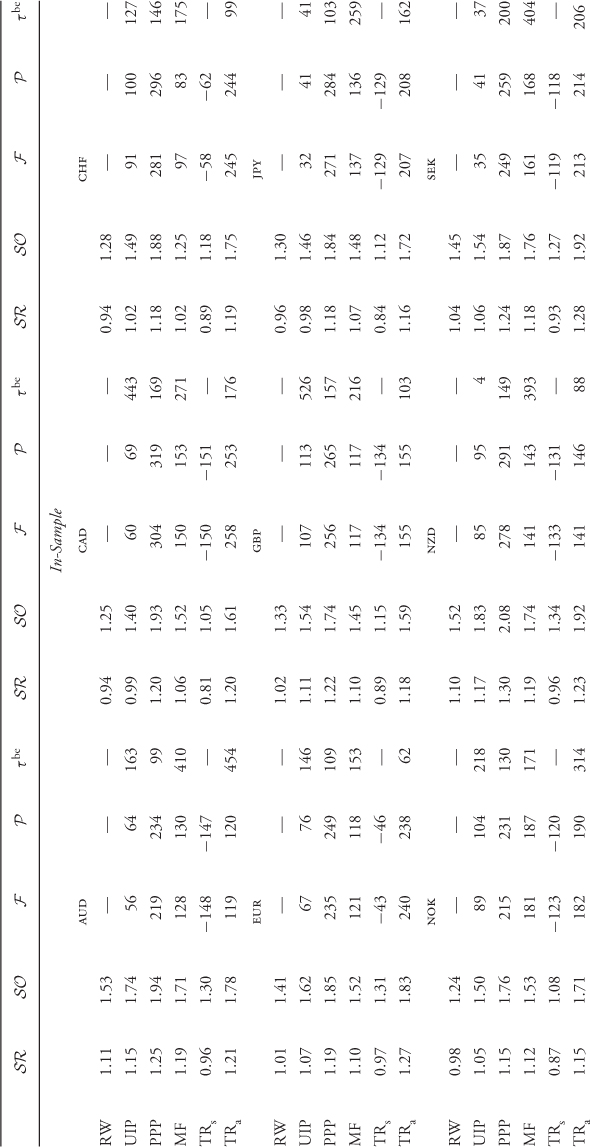
Table 8.7 shows the IS and OOS economic value of exchange rate predictability from the perspective of each of nine countries other than the US. For example, using the AUD as numeraire means that all exchange rates are quoted relative to AUD, all predictive regressions are estimated using the new exchange rates, and the mean-variance economic evaluation is done from the perspective of an Australian investor. The same holds when the numeraire changes to CAD, CHF, EUR, GBP, JPY, NOK, NZD, and SEK. We find that our main results remain robust across all numeraires: the best IS and OOS models are consistently the UIP, the PPP, and the TRa. In terms of Sharpe ratios and performance fees, in sample, the PPP and TRa outperform the RW for all nine numeraires and UIP does so six of nine times; OOS the PPP outperforms the RW seven of nine times, whereas the UIP and TRa five of nine times. To conclude, the economic value of exchange rate predictability of the best individual empirical exchange rate models remains robust regardless of the numeraire choice.
Table 8.7 The Economic Value of Exchange Rate Predictability for Alternative Numeraires
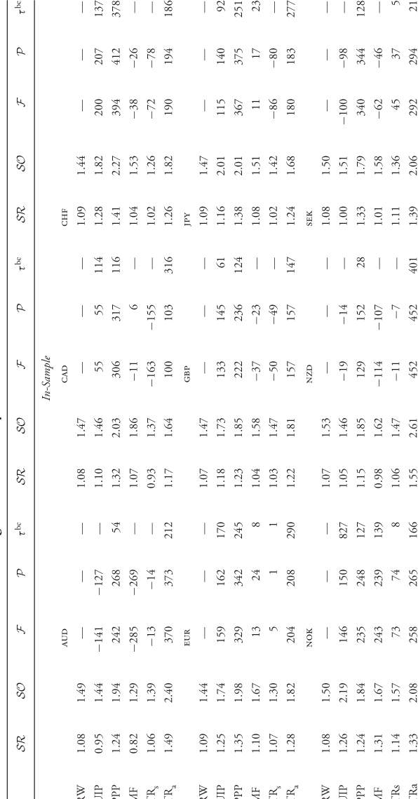

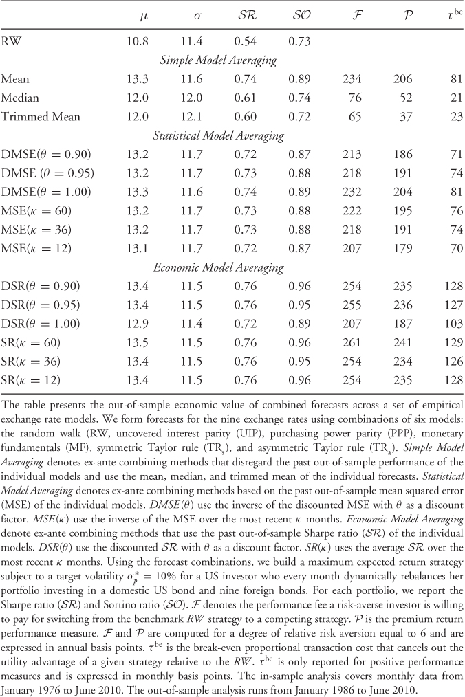
In addition to the results associated with individual models, even stronger economic evidence is found for the combined forecasts reported in Table 9.8. In all cases, forecast combinations significantly outperform the RW model. In fact, the best performing model averaging strategies are those based on the  . For example, the SR(κ = 12) strategy generates (i)
  compared to the RW where
  and (ii)
  annual bps with τbe = 128 monthly bps. It is noteworthy that the simple model average strategy using the mean forecast also generates a high
  and
and  bps. Another trend worth mentioning is that the degree of discounting (θ) or the length of the most recently best period (κ) have little or no effect on the performance of combined forecasts. In short, therefore, there is clear OOS economic evidence on the superiority of combined forecasts relative to the RW benchmark that tends to be robust to the way combined forecasts are formed. Finally, Figure 8.1 compares the OOS Sharpe ratios for the three best performing individual models (UIP, PPP, and TRa) and the SR(κ = 60) forecast combination with that of the RW.
Figure 8.1 Out-of-sample Sharpe ratios. The figure displays the out-of-sample annualized Sharpe ratio ( ) for selected empirical exchange rate models. We show the results from forming exchange rate forecasts using uncovered interest parity (UIP), purchasing power parity (PPP), asymmetric Taylor rule (TRa), and the ex-ante forecast combination method that uses the out-of-sample
  over the past 60 months (SR(κ = 60)). All models (solid line) are displayed versus the random walk (RW) benchmark (dashed line). Using the exchange rate forecasts from each model, we build a maximum expected return strategy subject to a target volatility
  for a US investor who every month dynamically rebalances her portfolio investing in a domestic US bond and nine foreign bonds. The
  is computed using the out-of-sample portfolio returns for one year. The out-of-sample period runs from January 1986 to June 2010.
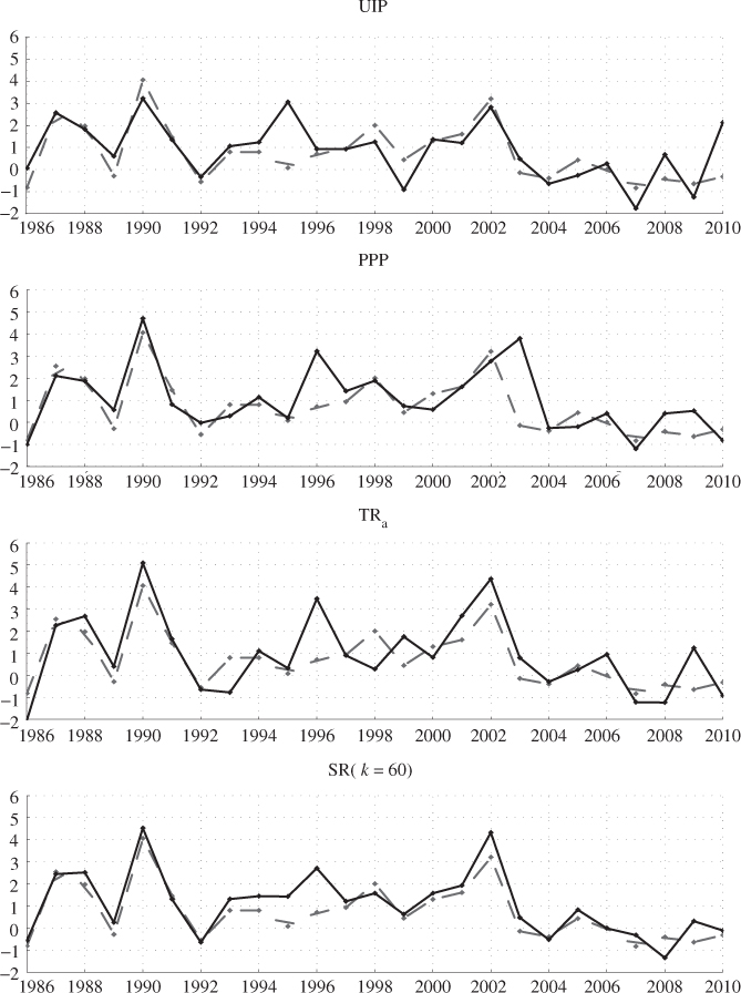
Table 8.8 The Economic Value of Combined Forecasts
Thirty years of empirical research in international finance has attempted to resolve whether exchange rates are predictable. Most of this literature uses statistical criteria for OOS tests of the null of the RW representing no predictability against the alternative of linear models that depend on economic fundamentals. The results of these studies are specific to, among other things, the empirical model and the exchange rate series. The emerging literature has moved in a different direction by providing an economic evaluation of predictability. This second line of research takes the view of an investor who builds a dynamic asset allocation strategy that depends on the forecasts from a set of empirical exchange rate models. The results of these studies are also specific to the empirical model, but instead of providing results for one exchange rate at a time, they evaluate predictability by looking at the performance of dynamically rebalanced portfolios. Finally, there is a third strand of empirical work that forms ex-ante combined forecasts from a set of individual empirical models. The results of these studies are not particular to an empirical model but rather relate to forecast combinations that account for model uncertainty.
This chapter reviews and connects these three loosely related literatures. We illustrate the statistical and economic methodologies by estimating a set of widely used empirical exchange rate models using monthly returns from nine major USD exchange rates. In line with Campbell and Thompson (2008), we show that modest statistical significance can generate large economic benefits for investors with a dynamic FX portfolio strategy. We find three main results (i) empirical models based on UIP, PPP, and the TRa perform better than the random walk in OOS forecasting using both statistical and economic criteria; (ii) depending on MF or using a symmetric Taylor rule does not generate economic value OOS; and (iii) combined forecasts formed using a variety of model averaging methods perform better than individual empirical models. These results are robust to reasonably high transaction costs, the choice of numeraire, and the exclusion of any one currency from the investment opportunity set.
This appendix summarizes the bootstrap algorithm we use for generating critical values for the OOS test statistics under the null of no exchange rate predictability against a one-sided alternative of linear predictability. Following Mark (1995) and Kilian (1999), the algorithm consists of the following steps:
 and the OOS period for
  . We generate P = (T − 1) − M OOS forecasts
  by estimating the predictive regression
and then computing the test statistic of interest,  .
.
and estimate this model subject to the constraint that β in the first equation is zero, using the full sample of observations  . The lag order p in the second equation is determined by a suitable lag order selection criterion such as the Bayesian information criterion (BIC).
 as follows:
The pseudo-innovation term  is randomly drawn with replacement from the set of observed residuals
  . The initial observations
  are randomly drawn from the actual data. Repeat this step B = 10, 000 times.
 , and an OOS period for
  . Then, generate P OOS forecasts
  by estimating the predictive regression
both under the null and the alternative for t = M + 1, … , T − 1, and construct the test statistic of interest,  .
.
 as
as
where I( · ) denotes an indicator function, which is equal to 1 when its argument is true and 0 otherwise.
The authors are grateful to Lucio Sarno and an anonymous referee for useful comments.
1The assumption of integrated fundamentals of order 1 is widely accepted in the literature. The assumption that the discount factor is close to 1 has been empirically validated by Sarno and Sojli (2009).
2Note that we will not be discussing two recent approaches to predicting movements in exchange rates: (i) the microstructure approach that depends on order flow as a measure of net buying pressure for a currency (Evans and Lyons, 2002; Rime et al., 2010) and (ii) the global imbalances approach (Gourinchas and Rey, 2007, and Della Corte et al., 2012).
3The argument still follows if the home country also targets exchange rates. It is standard to omit the exchange rate target from Equation (8.3) on the interpretation that US monetary policy has essentially ignored exchange rates (Engel and West, 2005).
4An alternative way of testing UIP is to estimate the “Fama regression” (Fama, 1984), which conditions on the forward premium. Note that if covered interest parity (CIP) holds, the interest rate differential is equal to the forward premium and testing UIP is equivalent to testing for forward unbiasedness in exchange rates (Bilson, 1981). For recent evidence on CIP see Akram et al. (2008).
5Clarida et al. (2003, 2006) and Boudoukh et al. (2006) also show that the term structure of forward exchange (and interest) rates contains valuable information for forecasting spot exchange rates.
6Note that in estimating the HP trend in sample or out of sample, at any given period t, we only use data up to period t − 1. We then update the HP trend every time, a new observation is added to the sample. This captures as closely as possible the information available to central banks at the time decisions are made.
7For a review of forecast evaluation, see West (2006) and Clark and McCracken (2011).
8The IS period for xt ranges from January 1976 to December 1985. The first OOS forecast is for the February 1986 value of Δst+1 that depends on the January 1986 value of xt. The last forecast is for June 2010.
9This approximation tends to perform better when forecasts are obtained from rolling regressions than recursive regressions.
10See Della Corte et al. (2012) for an economic evaluation of volatility and correlation timing in FX.
11In recent years, the typical transaction cost a large investor pays in the FX market is 1 pip, which is equal to 0.01 cent. For example, if the USD/GBP exchange rate is equal to 1.5000, 1 pip would raise it to 1.5001 and this would roughly correspond to 1/2 basis point proportional cost.
12Our empirical analysis uses the full bid-ask spread. Note, however, that the effective spread is generally lower than the quoted spread, since trading takes place at the best price quoted at any point in time, suggesting that the worse quotes will not attract trades. For example, Goyal and Saretto (2009) and Della Corte et al. (2011) consider effective transaction costs in the range of 50%–100% of the quoted spread. Assuming that the effective spread is less than the quoted spread would make our economic evidence stronger.
13The derivation is as follows  . Then,
  .
.
14For a slightly different calculation, see Jondeau and Rockinger (2008).
15For a Bayesian approach to forecast combinations, see Avramov (2002), Cremers (2002), Wright (2008), and Della Corte et al. (2009, 2012).
16Before the introduction of the euro in January 1999, we used the USD-Deutsche mark exchange rate combined with the official conversion rate between the Deutsche mark and the euro.
17For Germany, for the period January 1976 to December 1979, we construct the money supply using data on currency outside banks and demand deposits from IFS.
18For New Zealand, IPI data are only available from June 1977. We fill the gap using quarterly GDP data.
19The output gap for the first period is computed using real output data from January 1970 to January 1976. In the HP filter, we use a smoothing parameter equal to 14,400 as in Molodtsova and Papell (2009).
Abhyankar A, Sarno L, Valente G. Exchange rates and fundamentals: evidence on the economic value of predictability. J Int Econ 2005; 66: 325–348.
Akram F, Rime D, Sarno L. Arbitrage in the foreign exchange market: turning on the microscope. J Int Econ 2008; 76: 237–253.
Avramov D. Stock return predictability and model uncertainty. J Financ Econ 2002; 64: 423–458.
Bandi FM, Russell JR. Separating microstructure noise from volatility. J Financ Econ 2006; 79: 655–692.
Bandi FM, Russell JR, Zhu Y. Using high-frequency data in dynamic portfolio choice. Economet Rev 2008; 27: 163–198.
Bates JM, Granger CWJ. The combination of forecasts. Oper Res Q 1969; 20: 451–468.
Bilson JFO. The ‘Speculative Efficiency’ hypothesis. J Bus 1981; 54: 435–451.
Boudoukh J, Richardson M, Whitelaw RF. The information in long-maturity forward rates: implications for exchange rates and the forward premium anomaly. working paper, New York University; 2006.
Brunnermeier MK, Nagel S, Pedersen LH. Carry trades and currency crashes, NBER Macroeconomics Annual 2008; 2009. pp. 313–347.
Burnside C, Eichenbaum M, Kleshchelski I, Rebelo S. Do peso problems explain the returns to the carry trade? Rev Financ Stud 2011; 24: 853–891.
Campbell JY, Shiller RJ. Cointegration and tests of present value models. J Pol Econ 1987; 95: 1062–1088.
Campbell JY, Shiller RJ. Stock prices, earnings, and expected dividends. J Finance 1988; 43: 661–676.
Campbell JY, Thompson SB. Predicting excess stock returns out of sample: can anything beat the historical average? Rev Financ Stud 2008; 21: 1509–1531.
Cheung Y-W, Chinn MD, Pascual AG. Empirical exchange rate models of the nineties: are any fit to survive? J Int Money Finance 2005; 24: 1150–1175.
Clarida R, Gali J, Gertler M. Monetary policy rules in practice: some international evidence. Eur Econ Rev 1998; 42: 1033–1067.
Clarida RH, Sarno L, Taylor MP, Valente G. The out-of-sample success of term structure models as exchange rate predictors: a step beyond. J Int Econ 2003; 60: 61–83.
Clarida RH, Sarno L, Taylor MP, Valente G. The role of asymmetries and regime shifts in the term structure of interest rates. J Bus 2006; 79: 1193–1225.
Clark TE, McCracken MW. Tests of equal forecast accuracy and encompassing for nested models. J Economet 2001; 105: 85–110.
Clark TE, McCracken MW. Testing for unconditional predictive ability. In: Hendry D, Clements M, editors. Oxford handbook on economic forecasting. Oxford University Press; 2011. Forthcoming.
Clark TE, West KD. Using out-of-sample mean squared prediction errors to test the martingale difference hypothesis. J Economet 2006; 135: 155–186.
Clark TE, West KD. Approximately normal tests for equal predictive accuracy. J Economet 2007; 138: 291–311.
Cremers M. Stock return predictability: a bayesian model selection perspective. Rev Financ Stud 2002; 15: 1223–1249.
Della Corte P, Sarno L, Sestieri G. The predictive information content of external imbalances for exchange rate returns: how much is it worth? Rev Econ Stat 2012; 94: 100–115.
Della Corte P, Sarno L, Thornton DL. The expectation hypothesis of the term structure of very short-term rates: statistical tests and economic value. J Financ Econ 2008; 89: 158–174.
Della Corte P, Sarno L, Tsiakas I. An economic evaluation of empirical exchange rate models. Rev Financ Stud 2009; 22: 3491–3530.
Della Corte P, Sarno L, Tsiakas I. Spot and forward volatility in foreign exchange. J Financ Econ 2011; 100: 496–513.
Della Corte P, Sarno L, Tsiakas I. Volatility and correlation timing in active currency management. In: James J, Sarno L, Marsh IW, editors. Handbook of exchange rates. London: Wiley; 2012. Forthcoming.
Diebold FX, Mariano RS. Comparing predictive accuracy. J Bus Econ Stat 1995; 13: 253–263.
Engel C. The forward discount anomaly and the risk premium: a survey of recent evidence. J Empir Finance 1996; 3: 123–192.
Engel C, Mark NC, West KD. Exchange rate models are not as bad as you think. NBER Macroeconomics Annual 2007; 2007. pp. 381–441.
Engel C, West KD. Exchange rates and fundamentals. J Pol Econ 2005; 113: 485–517.
Evans MDD, Lyons RK. Order flow and exchange rate dynamics. J Pol Econ 2002; 110: 170–180.
Fama EF. Forward and spot exchange rates. J Monet Econ 1984; 14: 319–338.
Fleming J, Kirby C, Ostdiek B. The economic value of volatility timing. J Finance 2001; 56: 329–352.
Goetzmann W, Ingersoll J, Spiegel M, Welch I. Portfolio performance manipulation and manipulation-proof performance measures. Rev Financ Stud 2007; 20: 1503–1546.
Gomez V, Maravall A. Seasonal adjustment and signal extraction in economic time series. In: Pena D, Tiao GC, Tsay TR, editors. A course in time series analysis. New York: Wiley; 2000.
Gourinchas P-O, Rey H. International financial adjustment. J Pol Econ 2007; 115: 665–703.
Goyal A, Saretto A. Cross-section of option returns and volatility. J Financ Econ 2009; 94: 310–326.
Groen JJJ. The monetary exchange rate model as a long-run phenomenon. J Int Econ 2000; 52: 299–319.
Hai W, Mark NC, Wu Y. Understanding spot and forward exchange rate regressions. J Appl Economet 1997; 12: 715–734.
Han Y. Asset allocation with a high dimensional latent factor stochastic volatility model. Rev Financ Stud 2006; 19: 237–271.
Hodrick RJ. The empirical evidence on the efficiency of forward and futures foreign exchange markets. London: Harwood; 1987.
Hodrick RJ, Prescott EC. Postwar U.S. business cycles: an empirical investigation. J Money Credit Bank 1997; 29: 1–16.
Jondeau E, Rockinger M. Time-variability in higher moments is important for asset allocation. Unpublished Working paper, University of Lausanne; 2008.
Kilian L. Exchange rates and monetary fundamentals: what do we learn from long-horizon regressions? J Appl Economet 1999; 14: 491–510.
Lothian JR, Taylor MP. Real exchange rate behavior: the recent float from the perspective of the past two centuries. J Pol Econ 1996; 104: 488–509.
Mark NC. Exchange rates and fundamentals: evidence on long-horizon predictability. Am Econ Rev 1995; 85: 201–218.
Mark NC. Changing monetary policy rules, learning, and real exchange rate dynamics. J Money Credit Bank 2009; 41: 1047–1070.
Mark NC, Sul D. Nominal exchange rates and monetary fundamentals: evidence from a small post-bretton woods panel. J Int Econ 2001; 53: 29–52.
Marquering W, Verbeek M. The economic value of predicting stock index returns and volatility. J Financ Quant Anal 2004; 39: 407–429.
McCracken MW. Asymptotics for out of sample tests of granger causality. J Economet 2007; 140: 719–752.
Meese RA, Rogoff K. Empirical exchange rate models of the seventies: do they fit out of sample? J Int Econ 1983; 14: 3–24.
Molodtsova T, Papell DH. Out-of-sample exchange rate predictability with taylor rule fundamentals? J Int Econ 2009; 77: 167–180.
Neely CJ, Weller PA, Ulrich JM. The adaptive markets hypothesis: evidence from the foreign exchange market. J Financ Quant Anal 2009; 44: 467–488.
Nelson CR, Kim MJ. Predictable stock returns: the role of small sample bias. J Finance 1993; 48: 641–661.
Newey WK, West KD. A simple, positive semi-definite, heteroskedasticity and autocorrelation consistent covariance matrix. Econometrica 1987; 55: 703–708.
Orphanides A. Monetary policy rules based on real-time data. Am Econ Rev 2001; 91: 964–985.
Orphanides A, van Norden S. The unreliability of output gap estimates in real time. Rev Econ Stat 2002; 84: 569–583.
Rapach DE, Strauss JK, Zhou G. Out-of-sample equity premium prediction: combination forecasts and links to the real economy. Rev Financ Stud 2010; 23: 821–862.
Rime D, Sarno L, Sojli E. Exchange rate forecasting, order flow and macroeconomic information. J Int Econ 2010; 80: 72–88.
Rogoff KS. The purchasing power parity puzzle. J Econ Lit 1996; 34: 647–668.
Rogoff KS, Stavrakeva V. The continuing puzzle of short horizon exchange rate forecasting. NBER Working Paper No. 14071; 2008.
Sarno L. Towards a solution to the puzzles in exchange rate economics: where do we stand? Can J Econ 2005; 38: 673–708.
Sarno L, Sojli E. The feeble link between exchange rates and fundamentals: can we blame the discount factor? J Money Credit Bank 2009; 41: 437–442.
Stambaugh RF. Predictive regressions. J Financ Econ 1999; 54: 375–421.
Stock JH, Watson MW. Forecasting output and inflation: the role of asset prices. J Econ Lit 2003; 41: 788–829.
Stock JH, Watson MW. Combination forecasts of output growth in a seven-country data set. J Forecast 2004; 23: 405–430.
Taylor JB. Discretion versus policy rules in practice. Carnegie-Rochester Conf Ser Publ Policy 1993; 39: 195–214.
Taylor AM, Taylor MP. The purchasing power parity debate. J Econ Perspect 2004; 18: 135–158.
Timmermann A. Forecast combinations. In: Elliott G, Granger CWJ, Timmermann A, editors. Handbook of economic forecasting. Amsterdam: Elsevier; 2006.
Welch I, Goyal A. A comprehensive look at the empirical performance of equity premium prediction. Rev Financ Stud 2008; 21: 1455–1508.
West KD. Dividend innovations and stock price volatility. Econometrica 1988; 56: 37–61.
West KD. Asymptotic inference about predictive ability. Econometrica 1996; 64: 1067–1084.
West KD. Forecast evaluation. In: Elliott G, Granger CW, Timmermann A, editors. Volume 1, Handbook of economic forecasting. 2006. pp. 99–134. Chapter 3.
West KD, Edison HJ, Cho D. A utility-based comparison of some models of exchange rate volatility. J Int Econ 1993; 35: 23–45.
Wright JH. Bayesian model averaging and exchange rate forecasting. J Economet 2008; 146: 329–341.