The first script, log_adc.py, allows us to collect data and write it to a log file.
We can use the ADC device by importing data_adc as the dataDevice, or we can import data_local to use the system data. The numbers given to VAL0 through VAL3 allow us to change the order of the channels (and, if using the data_local device, select the other channels). We can also define the format string for the header and each line in the log file (to create a file with data separated by tabs) using %s, %d, and %f to allow us to substitute strings, integers, and float values, as shown in the following table:
When logging in to the file (when FILE=True), we open data.log in write mode using the 'w' option (this will overwrite any existing files; to append to a file, use 'a').
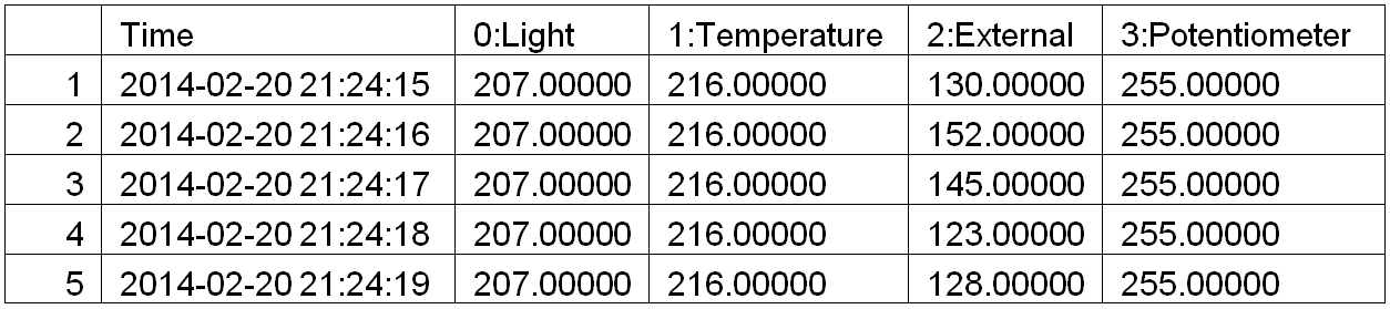
As part of our data log, we generate timestamp using time and datetime to get the current epoch time (this is the number of milliseconds since January 1, 1970) using the time.time() command. We convert the value into a more friendly year-month-day hour:min:sec format using strftime().
The main() function starts by creating an instance of our device class (we made this in the previous example), which will supply the data. We fetch the channel names from the data device and construct the header string. If DEBUG is set to True, the data is printed to the screen; if FILE is set to True, it will be written to the file.
In the main loop, we use the getNew() function of the device to collect data and format it to display on the screen or be logged to the file. The main() function is called using the try: finally: command, which will ensure that when the script is aborted, the file will be closed correctly.
The second script, log_graph.py, allows us to read the log file and produce a graph of the recorded data, as shown in the following diagram:

We start by opening up the log file and reading the first line; this contains the header information (which we can then use to identify the data later on). Next, we use numpy, a specialist Python library that extends how we can manipulate data and numbers. In this case, we use it to read in the data from the file, split it up based on the tab delimiter, and provide identifiers for each of the data channels.
We define a figure to hold our graphs, adding two subplots (located in a 2 x 1 grid at positions 1 and 2 in the grid - set by the values 211 and 212). Next, we define the values we want to plot, providing the x values (data['sample']), the y values (data['DATA0']), the color value ('r' for Red or 'b' for Blue), and label (set to the heading text we read previously from the top of the file).
Finally, we set a title and the x and y labels for each subplot, enable legends (to show the labels), and display the plot (using plt.show()).