Convolution is the central concept behind the CNN architecture. In simple terms, convolution is a mathematical operation that combines information from two sources to produce a new set of information. Specifically, it applies a special matrix known as the kernel to the input tensor to produce a set of matrices known as the feature maps. The kernel can be applied to the input tensor using any of the popular algorithms.
The most commonly used algorithm to produce the convolved matrix is as follows:
N_STRIDES = [1,1]
1. Overlap the kernel with the top-left cells of the image matrix.
2. Repeat while the kernel overlaps the image matrix:
    2.1 c_col = 0
    2.2 Repeat while the kernel overlaps the image matrix:
        2.1.1 set c_row = 0
        2.1.2 convolved_scalar = scalar_prod(kernel, overlapped cells)
        2.1.3 convolved_matrix(c_row,c_col) = convolved_scalar
        2.1.4 Slide the kernel down by N_STRIDES[0] rows.
        2.1.5 c_row = c_row  + 1
    2.3 Slide the kernel to (topmost row, N_STRIDES[1] columns right)
    2.4 c_col = c_col + 1
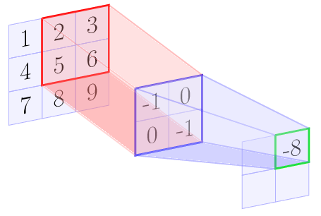
For example, let us assume the kernel matrix is a 2 x 2 matrix, and the input image is a 3 x 3 matrix. The following diagrams show the above algorithm step by step:
 |
 |
 |
 |
At the end of the convolution operation we get the following feature map:
| -6 | -8 |
| -12 | -14 |
In the example above the resulting feature map is smaller in size as compared to the original input to the convolution. Generally, the size of the feature maps gets reduced by (kernel size-1). Thus the size of feature map is :

The 3-D Tensor
For 3-D tensors with an additional depth dimension, you can think of the preceding algorithm being applied to each layer in the depth dimension. The output of applying convolution to a 3D tensor is also a 2D tensor as convolution operation adds the three channels.
The Strides
The strides in array N_STRIDES is the number the rows or columns by which you want to slide the kernel across. In our example, we used a stride of 1. If we use a higher number of strides, then the size of the feature map gets reduced further as per the following equation:

The Padding
If we do not wish to reduce the size of the feature map, then we can use padding on all sides of the input such that the size of features is increased by double of the padding size. With padding, the size of the feature map can be calculated as follows:

TensorFlow allows two kinds of padding: SAME or VALID. The SAME padding means to add a padding such that the output feature map has the same size as input features. VALID padding means no padding.
The result of applying the previously-mentioned convolution algorithm is the feature map which is the filtered version of the original tensor. For example, the feature map could have only the outlines filtered from the original image. Hence, the kernel is also known as the filter. For each kernel, you get a separate 2D feature map.
Convolution Operation in TensorFlow
TensorFlow provides the convolutional layers that implement the convolution algorithm. For example, the tf.nn.conv2d() operation with the following signature:
tf.nn.conv2d(
  input,
  filter,
  strides,
  padding,
  use_cudnn_on_gpu=None,
  data_format=None,
  name=None
)
input and filter represent the data tensor of the shape [batch_size, input_height, input_width, input_depth] and kernel tensor of the shape [filter_height, filter_width, input_depth, output_depth]. The output_depth in he kernel tensor represents the number of kernels that should be applied to the input. The strides tensor represents the number of cells to slide in each dimension. The padding is VALID or SAME as described above.
You can find more information on convolution layers available in Keras at the following link: https://keras.io/layers/convolutional/
The following links provide a detailed mathematical explanation of convolution:
http://colah.github.io/posts/2014-07-Understanding-Convolutions/
http://ufldl.stanford.edu/tutorial/supervised/FeatureExtractionUsingConvolution/
The convolution layer or operation connects the input values or neurons to the next hidden layer neurons. Each hidden layer neuron is connected to the same number of input neurons as the number of elements in the kernel. So in our previous example, the kernel has 4 elements, thus the hidden layer neuron is connected to 4 neurons (out of the 3 x 3 neurons) of the input layer. This area of 4 neurons of the input layer in our example is known as the receptive field in CNN theory.
The convolution layer has the separate weights and bias parameters for each kernel. The number of weight parameters is equal to the number of elements in the kernel, and only one bias parameter. All connections for the kernel share the same weights and bias parameters. Thus in our example, there would be 4 weight parameters and 1 bias parameter, but if we use 5 kernels in our convolution layer, then there would be total of 5 x 4 weight parameters and 5 x 1 bias parameters, a set of ( 4 weights, 1 bias) parameters for each feature map.