Now that we have the model, loss function, and optimizer function defined, train the model to learn the parameters, w, and b. To train the model, define the following global variables:
- num_epochs: The number of iterations to run the training for. With every iteration, the model learns better parameters, as we will see in the plots later.
- w_hat and b_hat: To collect the estimated w and b parameters.
- loss_epochs, mse_epochs, rs_epochs: To collect the total error value on the training dataset, along with the mse and r-squared values of the model on the test dataset in every iteration.
- mse_score and rs_score: To collect mse and r-squared values of the final trained model.
num_epochs = 1500
w_hat = 0
b_hat = 0
loss_epochs = np.empty(shape=[num_epochs],dtype=float)
mse_epochs = np.empty(shape=[num_epochs],dtype=float)
rs_epochs = np.empty(shape=[num_epochs],dtype=float)

mse_score = 0
rs_score = 0
After initializing the session and the global variables, run the training loop for num_epoch times:
with tf.Session() as tfs:
   tf.global_variables_initializer().run()
   for epoch in range(num_epochs):
Within each iteration of the loop, run the optimizer on the training data:
tfs.run(optimizer, feed_dict={x_tensor: X_train, y_tensor: y_train})
Using the learned w and b values, calculate the error and save it in loss_val to plot it later:
loss_val = tfs.run(loss,feed_dict={x_tensor: X_train, y_tensor: y_train})
loss_epochs[epoch] = loss_val
Calculate the mean squared error and r-squared value for the predicted values of the test data:
mse_score = tfs.run(mse,feed_dict={x_tensor: X_test, y_tensor: y_test})
mse_epochs[epoch] = mse_score

rs_score = tfs.run(rs,feed_dict={x_tensor: X_test, y_tensor: y_test})
rs_epochs[epoch] = rs_score
Finally, once the loop is finished, save the values of w and b to plot them later:
w_hat,b_hat = tfs.run([w,b])
w_hat = w_hat.reshape(1)
Let's print the model and final mean squared error on the test data after 2,000 iterations:
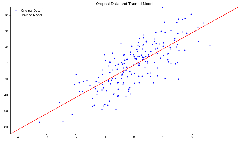
model : Y = 20.37448120 X + -2.75295663
For test data : MSE = 297.57995605, R2 = 0.66098368
Thus, the model that we trained is not a very good model, but we will see how to improve it using neural networks in later chapters.
The goal of this chapter is to introduce how to build and train regression models using TensorFlow without using neural networks.
Let's plot the estimated model along with the original data:
plt.figure(figsize=(14,8))
plt.title('Original Data and Trained Model')
x_plot = [np.min(X)-1,np.max(X)+1]
y_plot = w_hat*x_plot+b_hat
plt.axis([x_plot[0],x_plot[1],y_plot[0],y_plot[1]])
plt.plot(X,y,'b.',label='Original Data')
plt.plot(x_plot,y_plot,'r-',label='Trained Model')
plt.legend()
plt.show()
We get the following plot of the original data vs. the data from the trained model:
Let's plot the mean squared error for the training and test data in each iteration:
plt.figure(figsize=(14,8))

plt.axis([0,num_epochs,0,np.max(loss_epochs)])
plt.plot(loss_epochs, label='Loss on X_train')
plt.title('Loss in Iterations')
plt.xlabel('# Epoch')
plt.ylabel('MSE')

plt.axis([0,num_epochs,0,np.max(mse_epochs)])
plt.plot(mse_epochs, label='MSE on X_test')
plt.xlabel('# Epoch')
plt.ylabel('MSE')
plt.legend()

plt.show()
We get the following plot that shows that with each iteration, the mean squared error reduces and then remains at the same level near 500:

Let's plot the value of r-squared:
plt.figure(figsize=(14,8))
plt.axis([0,num_epochs,0,np.max(rs_epochs)])
plt.plot(rs_epochs, label='R2 on X_test')
plt.xlabel('# Epoch')
plt.ylabel('R2')
plt.legend()
plt.show()
We get the following plot when we plot the value of r-squared over epochs:

This basically shows that the model starts with a very low value of r-squared, but as the model gets trained and reduces the error, the value of r-squared starts getting higher and finally becomes stable at a point little higher than 0.6.