18
Applications and extensions of the Black-Scholes formula
In Chapter 16 we derived the so-called Black-Scholes formula, which gives compact and instructive expressions for the price of a call and of a put option in the Black-Scholes-Merton model. It turns out it is also possible to further apply and extend the Black-Scholes formula in various contexts, including financial products sold by insurance companies.
The aim of this chapter is mostly to analyze the pricing of options and other derivatives such as options on dividend-paying assets, currency options and futures options, but also insurance products such as investment guarantees, equity-indexed annuities and variable annuities, as well as exotic options (Asian, lookback and barrier options). In most of these cases, we can easily find a Black-Scholes-like formula for the no-arbitrage price of these contracts. The specific objectives of this chapter are to:
- use the Black-Scholes formula to price options on dividend-paying assets, currency options, futures options and exchange options;
- use financial engineering arguments and the Black-Scholes formula to obtain pricing formulas for investment guarantees, equity-indexed annuities and variable annuities;
- understand how to compute the break-even participation rate (annual fee) for common equity-linked insurance and annuities;
- derive the distribution of the discrete geometric mean of lognormally distributed random variables;
- understand why it might be difficult for various path-dependent options to obtain closed-form solutions;
- compute the price of average price Asian options (with a geometric mean), floating-strike lookback options and barrier options.
18.1 Options on other assets
In this section, we will derive analytic expressions for the price of options on dividend-paying stocks, currencies and futures in the BSM framework. We then conclude by analyzing exchange options when both assets are represented by a (joint, correlated) BSM model.
18.1.1 Options on dividend-paying stocks
We want to determine the no-arbitrage price of call and put options whenever a continuous dividend yield γ is paid by the underlying stock. Following Chapter 16, we will begin with a binomial tree defined over a time interval [0, T] that we divide into n sub-intervals of length T/n. The resulting tree is a n-step binomial tree in which the risky asset price, at any intermediate time k, is given by S(n)kT/n.
The main difference with Chapter 16 is that the tree now represents the evolution of the ex-dividend price, i.e. the price at which we can buy the asset on the market and upon which the option payoff is computed.
As usual, at maturity time T, i.e. when k = n, the (ex-dividend) asset price can be written as

where the number of up-moves  with
with

with respect to the actuarial probability measure  . Using the specifications of the Jarrow-Rudd tree, we have
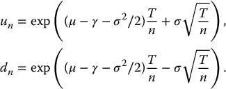
In contrast to Chapter 16, the mean rate of return on the stock is now μ − γ rather than just μ. Indeed, for k = 0, 1, …, n − 1,

so simplifications yield

A dividend is a cash outflow for the corporation and it slows down the growth of the ex-dividend stock price. However, a shareholder being entitled to these dividends, an investment of S(n)kT/n at time kT/n yields an expected return of μ − γ (from capital gains) plus a dividend yield of γ. Overall, the total expected return is μ.
As in Section 16.2.2, if the number of time steps goes to infinity (n → ∞), then

Note that this distribution is essentially the same as the one obtained in Section 16.2.2, i.e. when we had γ = 0, except that now, since dividends are paid, the parameter μ is replaced by μ − γ.
If we want to find the no-arbitrage price of a derivative, we have to determine the risk-neutral dynamics of the tree. The risk-neutral version of the Jarrow-Rudd tree, subject to dividend payments, is then based on the following parameters:
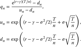
Thus, if n → ∞, at the limit we obtain the risk-neutral version of the distribution in (18.1.1):

To find the Black-Scholes formula with a continuous dividend yield γ, it suffices to compute, for 0 ⩽ t < T,

which is again the discounted stop-loss transform of a lognormal distribution. In this case, we must use the risk-neutral conditional distribution of ST (given St) which is

In conclusion, the Black-Scholes formula for a call option on a dividend-paying stock is, for all 0 ⩽ t < T,

where

Note that if γ = 0, then the classical Black-Scholes formula for a call option, as given in equation (16.3.3), is recovered.
Example 18.1.1 Call option price with a dividend yield
The initial price of a share of a dividend-paying stock is $34 with a continuous dividend yield of 1.25% per year. You know the stock price has a volatility of 27% and the risk-free rate is 4%. Compute the price of a 32-strike 6-month call option.
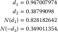
First, we compute d1(0, S0; γ) and d2(0, S0; γ) as given above: since γ = 0.0125, we have
Therefore, the formula for the call option price in (18.1.2) yields
◼
From the put-call parity relationship (when the underlying asset is paying continuous dividends) given in equation (6.4.6), we can deduce that the time-t value of the corresponding put option is

Using the Black-Scholes formula in (18.1.2), we get

Example 18.1.2 Put option price with a dividend yield
In the context of example 18.1.1, compute the value of the corresponding put option.
Using the Black-Scholes formula in (18.1.3), we find that P0 = 1.45157967. ◼
As in Section 16.6.2, the replicating portfolio of a call option written on a dividend-paying stock is already embedded in the Black-Scholes formula. Indeed, by inspection of the Black-Scholes formula given in (18.1.2), we see that the replicating portfolio is given by

where Δt is the number of units of the stock and where Θt is the number of units of the risk-free asset, both held at time t.
This is very similar to the replicating portfolio of a call option on a non-dividend-paying stock. The only difference with the case γ = 0 is the magnitude of the number of shares we should hold at time t: it is now e− γ(T − t)N(d1(t, St; γ)) shares instead of N(d1(t, St; 0)) shares. We can see that the number of shares of the stock needed in the replicating portfolio is smaller than in the case γ = 0. This is because dividends are reinvested in the stock. It also ensures the replicating strategy is self-financing; otherwise there would be a cash outflow.
Finally, it is important to note that in the BSM model, replication of options written on dividend-paying stocks requires continuous trading.
Example 18.1.3 Replicating a call on a dividend-paying stock
Consider again the setting of example 18.1.1. Initially, the replicating portfolio, as given in equation (18.1.4), is
In other words, at time 0, we buy 0.681894053 share of the stock at a (ex-dividend) price of $34 and we borrow $19.31101301.
We hold on to these quantities for the next 3 months, except for the reinvestment of dividends. This means that in 3 months we will hold 0.681894053 × e0.0125 × 0.25 shares of the stock.
Now, consider the following scenario: 3 months later, the stock price has increased to $36. Given that dividends have been reinvested in the stock, the investment in the stock has grown from 0.681894053 × 34 = 23.1843978 units to
The loan has grown with interest to
The portfolio value at time t = 0.25, i.e. 3 months later, but prior to rebalancing, is thus
This is in contrast with the call option price, which is in this scenario given by C0.25 = 4.643364432. Recall that the difference is the hedging error, which is a profit in this scenario.
◼
The replicating portfolio of a put option can also be obtained by identification. Inspecting the Black-Scholes formula in (18.1.3), we deduce that the replicating portfolio is, at any time 0 ⩽ t < T, given by

18.1.2 Currency options
We now analyze currency options which are options to buy or sell a foreign currency at a predetermined price. Recall from Section 12.3 that the notation is such that St corresponds to the price (expressed in the local currency) of one unit of the foreign currency.
Holding one unit of the foreign currency earns interest at the foreign risk-free rate rf. As seen previously in Section 12.3, a currency option can thus be viewed as an option on a dividend-paying stock with a dividend yield of rf. Therefore, the Black-Scholes formula for currency options is equivalent to equation (18.1.2) with γ = rf, i.e.

where d1(t, St; rf) and d2(t, St; rf) are as in equation (18.1.2) with rf taking the place of γ in the expression.
Example 18.1.4 Currency call option
You are a U.S. investor wishing to buy 1,000 Euros 3 months from now. Therefore, you enter into 1,000 3-month currency call options with a strike of 1.1 USD/EUR. You know that the risk-free rate in the U.S. is 2% whereas it is 3% in Europe. If the volatility on the exchange rate is 20% and the current exchange rate is 1.05 USD/EUR, calculate the amount required to buy those 1,000 call options.
We have r = 0.02, rf = 0.03, σ = 0.2, S0 = 1.05, K = 1.1. As of right now, buying one Euro costs S0 = 1.05 USD and we want to fix the buying price at K = 1.10 USD. Using the above Black-Scholes formula, we find that C0 = 0.02143608 per option and therefore the 1,000 options cost 21.43608. ◼
Replicating currency call options is similar to replicating options on dividend-paying stocks. Because the foreign currency earns interest at the foreign risk-free rate rf, the quantity of foreign currencies needed to replicate the payoff has to be smaller to account for this additional income.
18.1.3 Futures options and Black’s formula
Recall from Chapter 12 that a futures option is an option to buy or sell a futures contract at a predetermined price (which is different from the delivery/futures/forward price). In this section we will analyze options on futures (or futures options) in the BSM model, i.e. if the underlying asset price St follows the BSM dynamic. Note that in a binomial environment, we have modeled the futures price with a tree instead of the underlying asset price.
Assume that T⋆ is the maturity of a futures contract and T is the maturity of the futures option, with T⋆ ⩾ T. We know that, at time t, the T⋆-forward price of an asset is simply

First of all, note that

regardless of how ST and St are distributed. Since

for a non-dividend-paying stock, then

follows also a normal distribution but with different parameters:

The price of a futures option is then obtained by computing the usual conditional expectation

using the risk-neutral distribution of  given in equation (18.1.6). We can either evaluate the expectation using the stop-loss transform or simply let γ = r in equation (18.1.2) to obtain

where
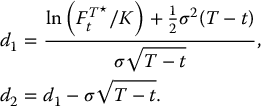
Equation (18.1.7) is also known as Black’s formula for a futures call option. A similar formula exists for a futures put option, i.e.

Example 18.1.5 Futures options
Futures on the S&P 500 index currently trade for 1200 whereas the volatility on the latter index is 18%. If the risk-free rate is 3%, find the price of 1-year at-the-money call and put options on that futures contract expiring after the options.
We have
and T = 1. Therefore, we obtain
Because the options are at the money, it is easy to remark that call and put options prices are exactly the same. Using Black’s formula, we see that
◼
18.1.4 Exchange options
Recall from Section 7.1.4, that an exchange option gives its holder the right to exchange an asset for another asset. Again, let us denote by S(1) and S(2) two risky assets whose price dynamics {S(1)t, t ⩾ 0} and {S(2)t, t ⩾ 0} are given by two dependent geometric Brownian motions. More precisely, the (real-world, actuarial) distributions of these prices are such that

and

where, for the i-th asset, μi and σi are the drift and diffusion coefficients and γi is the dividend yield, with i = 1, 2.
In a BSM environment, we assume that the random vector  has a bivariate normal distribution. The dependence structure (between these asset prices) is given through the correlation between the corresponding (normally distributed) log-returns, i.e.

To compute the no-arbitrage price of an exchange option, we know we will need to find the risk-neutral dynamics of these assets, that is, the risk-neutral distribution of the random vector  . It turns out that the log-returns have very similar real-world and risk-neutral distributions (and correlation), the only difference being that μ1 and μ2 are replaced by r in the latter. More precisely, the risk-neutral distributions of S(1) and S(2) are such that

where i = 1, 2, with correlation ρ as well.
From Section 7.1.4, the payoff of an option to obtain a share of S(1) in exchange for a share of S(2) at maturity T, is given by

Therefore, to derive the initial price of this exchange option, we need to compute

and the price at any time t is

However, the risk-neutral distribution of  , being the difference of two dependent and lognormally distributed random variables, is not easy to find. But if we condition on
  , then we can write

where the inside conditional expectation is easy to compute. Indeed, if we consider S(2)T or equivalently ln (S(2)T/S0) as a known value, then using a property of the bivariate normal distribution,1 the risk-neutral conditional expectation

can be computed using the Black-Scholes formula (or the stop-loss formula for lognormally distributed random variables), with the strike price replaced by S(2)T. The last (and tedious) step consists of taking the risk-neutral expectation of this modified Black-Scholes formula.
Finally, the price of this exchange option at any time t is given by

where

and where

It is interesting to note that the interest rate r does not appear in this formula.
Example 18.1.6 Consider a 1-year exchange option allowing to trade one share of ABC inc. for one share of XYZ inc. Both stocks currently sell for S(1)0 = S0(2) = 100. Let us find the initial price of this exchange option in a BSM environment with the following parameters: μ1 = 0.07, μ2 = 0.06, σ1 = σ2 = 0.2, γ1 = γ2 = 0 and ρ = −0.1.
In this case, the formula in (18.1.8) becomes
with
and
In conclusion,
Using the parity relationship seen in Section 7.1.4, we can also compute the exchange option allowing to get one share of S(2) in exchange for one share of S(1):
◼
Suppose now that S(2)T is an asset paying K with certainty at maturity T. It is easy to show that the no-arbitrage price of the exchange option to buy S(1) (with a dividend yield of γ1 = γ) in exchange for S(2) is the Black-Scholes formula for a call option on a dividend-paying asset.
If S(2)T = K (in all scenarios), then σ2 = 0, γ2 = 0 and S(2)t = Ke− r(T − t) at any time t. Using the pricing formula in equation (18.1.8), we find that

with
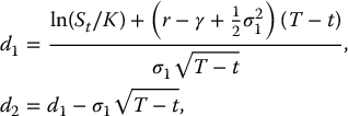
which is the classical Black-Scholes formula for a call option.
18.2 Equity-linked insurance and annuities
We would like to find the price of various equity-linked insurance and annuities (ELIAs), as introduced in Chapter 8, when the underlying follows a BSM dynamic. It is important to remember that finding the no-arbitrage price of a derivative assumes implicitly that agents are rational, i.e. they trade to optimize their gains and thus are ready to exploit any arbitrage opportunity if any. Does this apply to ELIAs typically sold to common people? Not so much.
However, no-arbitrage pricing matters as long as ELIAs are sold by many insurance companies in a competitive market. Indeed, from economic arguments, competition will drive prices down to the marginal cost. For ELIAs, the marginal cost represents the cost of the replicating portfolio and hence the corresponding no-arbitrage price.
Therefore, we will use Black-Scholes formulas for the pricing of ELIAs, when applicable. Note that when this is not possible, one can use simulation methods (see Chapter 19 for more details). We begin by analyzing investment guarantees, then we move on to equity-indexed annuities (EIAs) and variable annuities (VAs).
18.2.1 Investment guarantees
As seen in Chapter 8, an investment guarantee with payoff  plays an important role in life insurance as it forms the basis of many ELIA policies. We know from Chapter 6 that the payoff of an investment guarantee can be easily replicated with simple options:
- a call option and a risk-free investment, i.e.

- a put option and a share of the underlying asset, i.e.

Consequently, we can obtain the time-t value of an investment guarantee in two equivalent ways. Indeed:
- First, note that the time-t value of K guaranteed at time T is equal to e− r(T − t)K. Then, if we use the Black-Scholes formula for a call as given in (18.1.2), we obtain
(18.2.1)

- Second, note that the time-t value of a derivative paying ST is equal to e− γ(T − t)St. Indeed, buying e− γ(T − t) unit of the asset at time t, for a price of St, and then reinvesting the dividends in the asset until time T yields a final value of ST. Then, if we use the Black-Scholes formula for a put as given in (18.1.3), we obtain
(18.2.2)

As expected, the pricing formulas in (18.2.1) and (18.2.2) are equal.
Example 18.2.1 Investment guarantee in a BSM environment
In the BSM model, you are given:
- S0 = 10;
- σ = 0.25;
- r = 0.03;
- γ = 0.
How much should you pay at time 0 for a 5-year investment guarantee where 80% of the initial stock price is guaranteed? Also, analyze this product from the point of view of the insurance company.
In this case, since we have T = 5 and K = 0.8 × S0 = 8, we get
Using the pricing formula in (18.2.1), we find that
This means that an insured who invests (at inception) $10,685 in this product will receive (at maturity) the largest value between $8,000, the guaranteed amount and the accumulated value of $10,000 invested at time 0 in the underlying asset, i.e. 1,000 shares of S bought at time 0. Despite the name investment guarantee, there is still a risk of losing some money, i.e. the final payout could be less than the initial investment (not even taking into account the time value of money). To be entitled to the (upside) benefits of the risky investment, the insured/investor has to bear some (downside) risk; there is no arbitrage in this market.
On the other side of the transaction, the insurer will receive $10,685 (at inception), which corresponds to the cost for setting up a replicating portfolio, i.e. buying 100 shares of the stock and 100 put options (with strike price 8 and maturity 5 years). If these put options are not available on the market, the insurer can replicate each option with the Black-Scholes replicating strategy seen in Chapter 16. The insurer can also take this $10,685 to buy call options and lend at the risk-free rate, which is the other replicating strategy for an investment guarantee.
◼
18.2.2 Equity-indexed annuities
A variety of indexing schemes for EIAs has been presented in Chapter 8. We will analyze two of them in a BSM framework:
- point-to-point (PTP);
- compound periodic ratchet (CPR).
For these two schemes, we will obtain closed-form expressions for the no-arbitrage value of their benefits. However, for most indexing schemes, simulation methods are needed (see Chapter 19).
18.2.2.1 Point-to-point
In Chapter 8, we saw that the maturity benefit (payoff) of a PTP EIA is given by

where I is the initial investment, where 0 < β < 1 is the participation rate in the cumulative return over [0, T], namely RT = ST/S0 − 1, and where GT is the guaranteed amount at maturity (usually a fraction of the initial investment I). As the initial investment I can be factorized in the above expression, to simplify the presentation, we will now work per dollar invested, i.e. we will assume that I = 1. Therefore, the normalized maturity benefit, or per-dollar benefit, is now given by

Clearly, we can write

Thus, the payoff function is of the form max (a + bx, c) and we can use the following identity

as seen in Chapter 6. For the PTP indexing scheme, since we have a = 1 − β, b = β/S0 and c = GT, we can also write

if we set  .
.
Clearly, this EIA is equivalent to a position in β/S0 units of an investment guarantee, with guaranteed amount K just given, and a risk-free investment (bond with face value 1 − β). Consequently, using the pricing formula in equation (18.2.1), we deduce that the time-t value of the PTP EIA is given by

where  and where

Example 18.2.2 Point-to-point indexing method (continued)
In Example 8.2.1, we had a PTP indexing scheme with a participation rate of 80% in the cumulative return of the S&P 500. We know that the guarantee applies to 100% of the initial investment. If the S&P 500 index is modeled by a geometric Brownian motion, as in the BSM model, with S0 = 2200, σ = 0.215, γ = 0.01 and if the risk-free rate is r = 0.03, then let us find the initial value of this PTP EIA for an initial investment of $1.
We have β = 0.8, GT = 1 and T = 8. First of all, we compute
Second, the initial value
is given by
Finally,
Therefore, it costs $1.01 to provide the largest value between $1 at maturity and an investment of $1 growing at 80% of the cumulative return on the S&P 500 (per dollar invested by the insured). Unless the insurance company charges a separate premium of $0.01, this product is not viable, from the insurance company’s point of view. The insurance company could, for example, lower the participation rate to break even at least. We will come back to this issue later. ◼
18.2.2.2 Compound periodic ratchet
For the CPR indexing scheme, the maturity benefit is

where

To obtain compact formulas and to simplify the presentation, we will assume that:
- I = 1, to obtain normalized values or prices per dollar invested;
- T = n;
- GT ⩽ I, so that the outer maximum operator disappears;
- compounding of the return yk is annual.
Therefore, the benefit of a compound annual ratchet (CAR) scheme becomes

We are ready to derive the time-0 value of this benefit. As we are in a BSM model, the random variables  and
and  (for k1 ≠ k2) are log-increments of a GBM. We know from Chapter 14 that relative increments of a GBM over non-overlapping intervals are independent and lognormally distributed. Therefore, the value at time 0 of the benefit from this CAR scheme is given by

Therefore, using the independence between the yks, we have
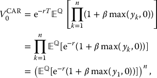
where in the last equality we used the fact that the yks have the same distribution (e.g. the distribution of y1).
Inside the expectation, we have

and then

Defining

which is the initial value of a one-year at-the-money call option on S, we obtain2

Finally, in the BSM model, an explicit expression for  is given by the Black-Scholes formula:

where

Example 18.2.3 Value of a CAR scheme
Find the initial value of a 10-year CAR scheme where the participation rate is 75%. Assume the CAR is written on a non-dividend paying asset whose volatility is 20%. Use a BSM model with a risk-free rate of 4% and suppose GT ⩽ I.
We compute
Therefore,
To provide the greatest between $10,000 (if the annual return on the stock is negative for each of the 10 years) and $10,000 accumulated with the latter ratcheting scheme costs $14,137. It is the replication value for the insurer. If the policyholder invests $10,000, the insurance company is likely to suffer an important loss.
This product seems too expensive: will an investor be willing to pay $14,137 and be guaranteed to receive at least $10,000? The company could lower the participation rate to bring these two quantities (initial value and guaranteed amount) closer to each other, as we will see below.
◼
18.2.2.3 Break-even participation rate
For the products described in examples 18.2.2 and 18.2.3, the cost of replicating their maturity benefits was larger than the initial investment made by the policyholder. Unless the policyholder is willing to pay an extra premium at inception, upon which no guarantee applies (0.01 per dollar invested in example 18.2.2, or 0.41 per dollar invested in example 18.2.3), these products are not very attractive for an investor, at least at first sight.
Instead of requiring an extra upfront premium, insurance companies can adjust the participation rate3 β so that the initial investment I = 1 covers the replication cost of the indexing scheme. In other words, we need to find β such that

where V0 is the initial value of the contract, e.g.  or
or  . Note that we have emphasized the fact that V0 depends on the value of the parameter β by writing V0(β). This notation means that all other quantities involved in the pricing formula stay fixed when β varies, especially the guaranteed amount. This value of β is known as the break-even participation rate. Most of the time, the solution to such an equation (the break-even participation rate) can only be found numerically using a root-finding algorithm.
However, for the CAR scheme described above, it is possible to solve this equation analytically. We want to find the value of β such that

We easily find that the break-even participation rate is given by

Example 18.2.4 (High) Value of a CAR scheme (continued)
Let us find the break-even participation rate in the CAR scheme of example 18.2.3. We easily find
The break-even participation rate is about 40%, which is much lower than the initial 75%.
Let us further analyze this product and its risk-return characteristics from the perspective of the policyholder. With a participation rate of 40%, the annual return on the underlying index should be more than 10% to compete with the risk-free rate of 4%. In other words, over this 10-year period, the CAR indexing scheme will generate more value than the guaranteed amount if the index constantly earns more (or much more) than 10%. In fact, the likelihood of accumulating more than 10000erT = 14918.25 by investing in this CAR scheme is about 55% (since μ = 0.08).4 This analysis highlights the fact that there is a high hidden cost to the minimum annual guaranteed return of 0%.
◼
18.2.3 Variable annuities
It is also possible to find explicit no-arbitrage values for variable annuities with a GMMB or a GMDB rider in a BSM framework. Just like the PTP indexing scheme, we will be able to rewrite the benefits in terms of investment guarantees. As for the valuation of a GMWB or a GLWB, one would need to use simulations (see Chapter 19) or other numerical schemes.
18.2.3.1 GMMB
In a GMMB, the sub-account balance evolves with credited returns whereas fees are deducted constantly. The policyholder is typically not allowed to make withdrawals and we will assume there are no deaths occurring prior to maturity.
In the BSM framework, we assume that the sub-account balance is adjusted continuously and thus

where the annual fee α is withdrawn continuously. Over the time interval [t, T], the sub-account accumulates according to

Given that the distribution of the accumulation factor ST/St is

we deduce that the sub-account balance is such that

(under the real-world/actuarial probability measure  ). For no-arbitrage pricing purposes, we also need to find the risk-neutral distribution of the sub-account balance. With similar steps, we obtain

(under the risk-neutral/pricing probability measure  ).
).
In other words, it is possible to view the dynamics of the sub-account balance as that of a dividend-paying asset with a continuous dividend yield of α. The fees paid by the insured act as a sort of dividend for the insurer. Indeed, from the policyholder’s perspective, the sub-account balance is like the ex-dividend price of an asset. Since the insurance company holds the sub-account in the name of the insured and therefore collects the fees, this is similar to holding a dividend-paying asset (which entitles its holder to capital gain and dividends).
In Chapter 8, we have seen that the maturity benefit of a GMMB is

with GT being defined similarly as in the context of EIAs. The maturity benefit is thus equivalent to an investment guarantee with the difference that the underlying asset is the sub-account balance. However, in this case, the sub-account is not a traded asset. Note that the dynamics of At is that of a GBM with a dividend yield α. Therefore, the GMMB is an investment guarantee on a dividend-paying asset whose time-t value is given by equation (18.2.1). Consequently, we have

with K replaced by GT, and with γ replaced by α. More precisely, we have

It is important to note that  is the initial cost for the insurance company to replicate this product and this replicating procedure relies on the inflow of fee payments (they are immediately reinvested in the replicating portfolio). Said differently, the initial value
  takes into account the amount of accumulated fees collected by the insurance company during the life of this product.
This is significantly different from the pricing of standard financial derivatives where a single premium is collected at inception by the seller. For variable annuities, in particular for GMMB riders, the insurance company collects the initial investment I as well as fee payments at rate α during the life of the contract.
Example 18.2.5 Initial value of a GMMB
Suppose that a policyholder enters into a 10-year GMMB such that the guaranteed amount at maturity corresponds to the initial investment. The sub-account credits the returns of an asset following a BSM dynamic with parameters μ = 0.07, σ = 0.25 and r = 0.02 and an annual fee rate of α = 2.5% is deducted continuously. Compute the initial value of the GMMB if the initial investment is $1.
In this case, we have T = 10 and A0 = I = 1 = G10. To use the Black-Scholes formula of equation (18.2.3), we need:
Therefore, the value of the GMMB at inception is
To provide this protection on the sub-account balance, the insurance company needs $1.044745885 per dollar invested by the policyholder. With an initial investment of $1 and a fee rate of 2.5% per annum, this GMMB is thus worth $1.044745885 to the policyholder. This means it is sold at a loss by the insurance company. In conclusion, the annual fee charged by the company is too low or the guaranteed amount is too high. ◼
18.2.3.2 GMDB
When a guarantee applies upon death of the policyholder, we know from Chapter 8 that this is a GMDB rider. Therefore, to protect an invested capital upon death or maturity, whichever comes first, one needs to combine both protections.5
If we knew in advance when the policyholder will die, we could treat the GMDB as a GMMB with a maturity corresponding to the time of death. This is (fortunately) not possible in practice. In this case, the insurance company can sell GMDBs to a very large number of independent and identically distributed (iid) policyholders so that the insurer can predict with a high probability the number of policyholders surviving each year. Consequently, we can treat a very large portfolio of GMDBs with each policy having a random effective maturity as a portfolio of GMMBs with deterministic maturities.
Suppose the insurance company holds a portfolio of M iid policyholders (e.g. all aged x) and let us denote Mk as the expected number of deaths from the pool in the k-th year. In practice, the real number of deaths should be different from its expectation, but with M large enough, the relative variability (Mk/M) should be small enough to be ignored.
Then, we know that selling T-year GMDBs to these M policyholders (assume T is an integer for the sake of the illustration) is roughly equal to holding a portfolio of:
- M1 1-year GMMBs whose maturity benefit is replaced by the death benefit that would apply at the end of year 1;
- M2 2-year GMMBs whose maturity benefit is replaced by the death benefit that would apply at the end of year 2;
- …;
- MT T-year GMMBs whose maturity benefit is replaced by the death benefit that would apply at the end of year T.
Let  be the initial value of a GMMB as given in (18.2.3) with an emphasis on the fact that it is maturing in k years with maturity guarantee Gk. Therefore, the total initial value of the GMDBs sold to the pool of policyholders is

The initial value of such a GMDB for a single policyholder is thus given by the total amount in (18.2.4) divided by the number of participants M in the pool, i.e.

Note that {M1/M, M2/M, …, MT/M} is a discrete probability distribution (w.r.t. the real-world/actuarial probability  ) over {1, 2, …, T} linked to the mortality distribution of these insureds. Consequently,
  is given by the average of the values
  weighted by this mortality distribution.
More generally, if we let τ be the random variable representing the time of death of a given policyholder, we would have the following general relationship:

It is very important to note that the expectation is taken with respect to the actuarial probability distribution of τ, which can be computed for example with a mortality table corresponding to the insureds common profile.
18.2.3.3 Break-even fee rate
In example 18.2.5, we found that the cost of replicating the maturity benefit was greater than what was received by the insurance company from the policyholder, at inception (initial investment) and from the sub-account (fees). Just like for EIAs, for which we found a break-even participation rate, we can find a break-even fee rate for variable annuities, given a guaranteed amount GT. As before, the idea is to determine the value of α such that

where V0 is the initial value of the contract, e.g.  or
or  .
.
Again, in most cases, the solution to such an equation (the break-even fee rate) can only be found numerically using a root-finding algorithm.
Example 18.2.6 Annual fee in a GMMB
Let us find the break-even annual fee rate α for the GMMB in example 18.2.5. We need to determine the value of α such that
since A0 = 1. Using for example the Goal Seek tool from ExcelTM, we find α = 0.034954116, i.e. the fee rate needs to be at least 3.5%, which is higher than the rate of 2.5% used in example 18.2.5.
Instead, if we assume the policyholder is willing to bear a 25% loss over 10 years, meaning that we now set GT = 0.75 × A0, then the break-even annual fee rate drops to α = 1.2575606%. ◼
18.3 Exotic options
Recall from Chapter 7 that a European payoff VT is said to be exotic or path-dependent if it depends on the underlying asset price at more than one date during the life of the derivative. There are two types of path-dependent payoffs determined by the monitoring frequency of the option:
- discretely monitored: for n ⩾ 2 and for a set of dates 0 ⩽ t1 < t2 < … < tn ⩽ T, the payoff is given by

- continuously monitored: the payoff is given by

These options are also said to be exotic to contrast with vanilla/simple options such as standard call and put options.
The main objective of this section is to derive formulas for the initial price of two types of exotic options: average price Asian options (with geometric mean) and floating-strike lookback options. By focusing on these options, we will be able to obtain Black-Scholes-like expressions that are easy to manipulate and to compute. As for barrier options, to derive expressions for their initial prices, more advanced mathematical techniques are needed; we will simply state the pricing formulas.
18.3.1 Asian options
We know from Chapter 7 that Asian options are derivatives whose payoff depends on the average asset price observed between inception and maturity. There are many types of Asian options depending on:
- how often the underlying asset price is monitored (discrete or continuous monitoring);
- how the average is computed (arithmetic or geometric average);
- how the average is used in the calculation of the payoff (average price or average strike).
In general, there are no simple formulas for the initial value of average strike Asian options. This is because we can buy or sell the underlying asset for an average strike of  and hence we need to determine the (risk-neutral) joint distribution of
  . Moreover, average price Asian options computed with an arithmetic average are also difficult to evaluate because we need to find the distribution of the sum of asset prices. Hence, for many Asian options, simulation methods are needed (see Chapter 19).
There is one case where we can obtain closed-form expressions for the initial price of an average price Asian option in the BSM model: when the average is geometric, computed either discretely or continuously. Recall that the payoff of these Asian options is given by

where the geometric average price  can be computed continuously or discretely. More precisely, the geometric average price of S is given by

in the continuous monitoring case, and by

for given dates 0 ⩽ t1 < t2 < … < tn ⩽ T, with n ⩾ 1, in the discrete monitoring case.
In a BSM setting, Asian options based on geometric averages are more tractable because the lognormal distribution is stable under multiplication (the product of independent lognormal random variables is also lognormally distributed). This is not the case when arithmetic averages are used.
Therefore, in what follows, we first analyze the distribution of the geometric average  . We will find that both the real-world/actuarial distribution and the risk-neutral distribution of the average are lognormally distributed. Second, we will use the stop-loss transform formula for lognormal random variables to obtain explicit formulas similar to the Black-Scholes formula.
18.3.1.1 Discrete geometric average
Let us begin by considering a simple case: the discrete geometric average  , i.e. the discrete geometric average of a geometric Brownian motion sampled at only two evenly-spaced dates. We know that at any time t, we have

Therefore, the product of ST/2 and ST is equal to

However, the random variables ST/2 and ST are not independent because WT/2 and WT have a non-zero covariance. Indeed, recall from Chapter 14 that the covariance between WT/2 and WT is given by  .
.
On the other hand, the random variables WT − WT/2 and WT/2 are independent because they are Brownian increments over non-overlapping time intervals. Consequently,

follows a normal distribution with mean 0 and variance 5T/2 (with respect to  ).
).
Taking the square root of the product, we obtain

and we get

More generally, if the average is based on n given dates 0 ⩽ t1 < t2 < … < tn ⩽ T, then we can write

where the random vector  follows a multivariate normal distribution. Consequently, ∑ni = 1Wti follows a (univariate) normal distribution with mean

and variance

Consequently, the geometric average follows a lognormal distribution:

Example 18.3.1 Probability of expiring in the money
A share of stock currently trades for $50 and a 1-year 51-strike average price Asian call option with geometric average is issued. If the average is computed over monthly prices, then calculate the probability the option matures in the money in a BSM model with μ = 0.08, r = 0.02, σ = 0.25.
We have ti = i/12, for each i = 1, 2, …, 12, and we have tn + 1 − i = (12 + 1 − i)/12 = (13 − i)/12. Therefore,
and
The probability of the option maturing in the money, i.e. the probability the payoff
is positive, is computed using the actuarial distribution of equation (18.3.1) (i.e. with the real-world probability
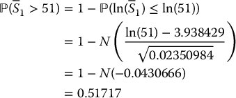
). We have
and
Finally,
is the probability for this Asian option of expiring in the money. ◼
18.3.1.2 Continuous geometric average
The continuous geometric average of S over the time interval [0, T] is defined by

Let {Xt, t ⩾ 0} be the linear Brownian motion with drift  and diffusion σ, i.e.

such that we can write  and ln (St) = ln (S0) + Xt. Hence, the continuous geometric average can be written as follows:

Since

using tools from stochastic calculus (see Chapter 15), we could verify that

and therefore

In conclusion, the continuous geometric average of a geometric Brownian motion also follows a lognormal distribution (with respect to  ). More specifically, we have

Example 18.3.2 Probability of expiring in the money (continued)
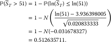
Let us assume now that the average is computed continuously. From equation (18.3.2),
follows a lognormal distribution with parameters
and
Consequently, the probability of the option maturing in the money is
◼
18.3.1.3 Black-Scholes formulas
We just showed that the geometric average of a geometric Brownian motion follows a lognormal distribution whose parameters depend on the monitoring frequency (discrete or continuous); see equation (18.3.1) and equation (18.3.2).
Now, we are interested in finding the no-arbitrage value of an average price (fixed-strike) Asian call option. This requires the computation of

which is a discounted stop-loss premium whose expectation is computed with the risk-neutral distribution (risk-neutral pricing probability  ). Therefore, we cannot directly use the results from equations (18.3.1) and (18.3.2)) as they are based on the actuarial distribution of asset prices.
Relying on the mathematical tools developed in Section 17.2 of Chapter 17,6 it turns out that the risk-neutral distribution of the geometric average is also lognormal:

in the discrete case, and

in the continuous case. The risk-neutral distributions in (18.3.3) and (18.3.4) are equivalent to those in (18.3.1) and (18.3.2) with μ replaced by r.
Therefore, we can say that  follows a risk-neutral lognormal distribution, i.e.

where m and s2 are given by either the expressions in (18.3.3) or in (18.3.4), depending on the monitoring frequency. It follows from formula (14.1.7) in Chapter 14 that

It is the Black-Scholes formula for the initial value of an average price Asian call option.
Example 18.3.3 Average price Asian call option
Your company sells an average price Asian call option with a strike price of $34 maturing in 4 months. The behavior of the stock price is such that its log-return volatility is 30%, its current price is $36 and the dynamics is that of the BSM model. Compute the price of the latter Asian call option if the average is computed continuously and the risk-free rate is 2%.
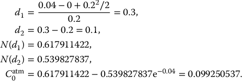
We have S0 = 36, K = 34, T = 0.25, σ = 0.3 and r = 0.02. We compute the parameters m and s2 of the risk-neutral lognormal distribution for the continuous geometric mean
given in (18.3.4): we get
The price of the option is thus given by the formula in (18.3.5):
◼
We know that

Therefore, we can deduce that the initial value of an average price Asian put option is such that

where

Again, m and s2 are given by the expressions in (18.3.3) or in (18.3.4), depending on the monitoring frequency. This is the parity relationship for average price Asian options.
Example 18.3.4 Average price Asian put option
Using the context of the previous example, find the price of the corresponding average price Asian put option.
Since
we get
◼
18.3.2 Lookback options
We know from Chapter 7 that lookback options are derivatives whose payoff depends on the minimum or maximum price of the underlying asset observed during the life of the option. The types of lookback options are based upon:
- how often the underlying asset price is monitored (discrete or continuous monitoring);
- how the maximum/minimum is used in the calculation of the payoff (as the underlying asset price or as the strike price).
There are closed-form expressions for the no-arbitrage price of lookback options when the minimum or maximum is monitored continuously. For simplicity, in what follows, we will discuss only floating-strike lookback options (see below).
18.3.2.1 Distribution of the maximum and the minimum
First, let us analyze the distribution of the maximal and minimal values taken by S in a BSM setting, in which case S is a geometric Brownian motion. Recall from Chapter 7 the definitions of the following random variables:

They are respectively the maximal value and the minimal value taken by the underlying asset price S over the time interval [0, T].
As the asset price is given by St = exp (Xt), where

i.e. where X is a linear Brownian motion with drift  and diffusion σ, if we define

then, since the exponential function x↦exp (x) is an increasing function, we have that

In words, the maximum (or minimum) value taken by the geometric Brownian motion S can be rewritten in terms of the maximum (or minimum) taken by the underlying Brownian motion with drift X. Consequently, the distribution of MST (resp. mST) is equivalent to finding the distribution of MXT (resp. mXT).
It is known7 that, for x > 0,

and, for x < 0,

where a = μ − σ2/2. Consequently, using the relationships presented above, we can write

and

18.3.2.2 Black-Scholes formulas
In a BSM model, the payoff of a floating-strike lookback put option is given by PfST = MST − ST, so its no-arbitrage initial price can be written as

The problem amounts to finding the expected value of the maximum using the risk-neutral distribution of the stock price (i.e. with the pricing probability  ).
).
Since MST is a positive random variable, its expectation is equal to the integral of its survival function, i.e.

The risk-neutral distribution of MST is slightly different from the real-world distribution in (18.3.6), as it is based on the risk-neutral dynamic of the linear Brownian motion X. It can be shown that, for x > 0,

where a = r − σ2/2 is used instead of μ − σ2/2. Finally, the price of the floating-strike lookback put option is found by integrating the risk-neutral survival function of MST, i.e. the function  over the interval (0, ∞), with the help of the expression given in (18.3.8).
Similarly, for a floating-strike lookback call option with payoff CfST = ST − mST, we have

where

Again, it can be shown that, for x < 0,

The expression in (18.3.9) can be used directly to derive the price of the call option.
As the final computations are tedious, for both lookback options we provide the pricing formulas without proof. First, let us define
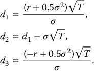
The initial value of the lookback call option is

whereas the initial value of the lookback put option is

18.3.3 Barrier options
We know from Chapter 7 that barrier options are derivatives whose payoff is activated or deactivated if the asset price crosses a predetermined barrier before maturity. Finding the no-arbitrage price of barrier options in the BSM framework is not easy: it requires the knowledge of the joint distribution of (ST, MST) or (ST, mST). In what follows, we will provide Black-Scholes-like pricing formulas for barrier options without proof.
Recall from Chapter 7 that there are four types of barrier options: up-and-in, up-and-out, down-and-in and down-and-out barrier options. Pricing formulas also depend on the relationship between the barrier level H and the strike price K, so that overall there are 16 possible combinations. To lighten the presentation, we will use the fact that a knock-in barrier option combined with the corresponding knock-out barrier option has the same payoff as a regular option.
18.3.3.1 Call options
Using the same acronyms as in Chapter 7 to name the different barrier call options, let us denote their initial prices by  ,
,  ,
,  and
and  . We do not recall the payoffs here, as they can be found in Chapter 7.
Let us begin with the case where the initial price S0 is above the trigger level H, i.e. S0 ⩾ H, meaning the asset price must go under H at some point for the barrier calls to be knocked-in or knocked-out.
If we further assume S0 ⩾ H ⩾ K, we can show that

where
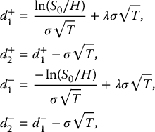
and where

Recalling from Chapter 7 that

we can conclude that  , where C0 is the initial price of a vanilla call option, as given by the Black-Scholes formula.
Instead, if we further assume H ⩽ K, which means now that S0 can be either greater than or less than the strike price K, then we can show that

where

and the corresponding down-and-out call option is such that  .
.
Now, let us consider the case where the initial price S0 is below the trigger level H, i.e. S0 ⩽ H, meaning the asset price must go above H at some point for the barrier options to be knocked-in or knocked-out.
If we further assume H ⩾ K, i.e. if S0 ⩽ K ⩽ H or if K ⩽ S0 ⩽ H, then we can show that

and the corresponding up-and-out call option is such that  .
.
Finally, if we further assume S0 ⩽ H ⩽ K, it is easy to see that  as its payoff will be equal to zero in all possible scenarios. Indeed, for the barrier call to mature in the money, i.e. to have ST > K, the underlying asset price must go above H during the life of the option and, by doing so, will be knocked-out. Therefore, in this case, we have
  .
.
18.3.3.2 Put options
We follow similar steps to present the various formulas for barrier put options. Again, using the same acronyms as in Chapter 7 to name the different barrier put options, let us denote their initial prices by  ,
,  ,
,  and
and  .
.
Let us begin with the case where the initial price S0 is above the trigger level H, i.e. S0 ⩾ H, meaning the asset price must go under H at some point for the barrier puts to be activated or deactivated.
If we further assume S0 ⩾ H ⩾ K, it is easy to see that  as its payoff will be equal to zero in all possible scenarios. Therefore, in this case, we have
  , where P0 is the initial price of a vanilla put option, as given by the Black-Scholes formula.
If we further assume H ⩽ K, i.e. if H ⩽ K ⩽ S0 or if H ⩽ S0 ⩽ K, then we have

and then  .
.
Now, let us consider the case where the initial price S0 is below the trigger level H, i.e. S0 ⩽ H, meaning the asset price must go above H at some point for the barrier options to be knocked-in or knocked-out.
If we further assume H ⩾ K, i.e. if S0 ⩽ K ⩽ H or if K ⩽ S0 ⩽ H, then we have

and then  .
.
Finally, if we further assume S0 ⩽ H ⩽ K, then

and then  .
.
18.4 Summary
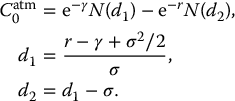
Options on other assets- Black-Scholes formula for a call option on an asset paying continuous dividends with yield γ:
with


- Replication portfolio for a call option on an asset paying continuous dividends with yield γ:

- Currency options: in the above formulas, interpret St as the price (expressed in the local currency) of one unit of the foreign currency and set γ = rf.
- Futures options: in the above formulas, assume the maturity of the futures T⋆ ⩾ T, replace St by
 and set γ = r. The pricing formula of a futures call option is known as Black’s formula.
 - Using put-call parity, we obtain the corresponding put option prices.
- Exchange option: the Black-Scholes formula of an option to buy S(2) in exchange for S(1) is:
where

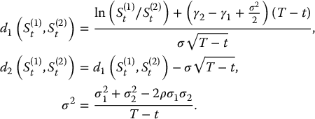
- The Black-Scholes formula for an investment guarantee with payoff max (ST, K) is:

- The Black-Scholes formula for a PTP EIA is:

- CAR: if we assume GT ⩽ I and T = n is an integer, then the price of a CAR is:
with

- The Black-Scholes formula for a GMMB is:
where


- GMDB: if we have a large portfolio of iid policyholders, we can view a GMDB as a portfolio of GMMBs with varying maturities given by the expected number of deaths.
- Asian options: when average is geometric, we have closed-form formulas.
- Lookback options: for floating-strike lookback options, we have closed-form formulas.
- Barrier options: in all cases, we have Black-Scholes-like formulas.
18.5 Exercises
In the following problems, assume the market is a Black-Scholes-Merton model.
-
Working for a U.S. insurance company, you are holding 1,000 Euros (EUR) and you will have to sell them 6 months from now. The current exchange rate is quoted at 1.05 USD/EUR and you are afraid the exchange rate will attain parity or worse be lower. Therefore, you seek to buy 1,000 put options at a strike of 1 USD (per Euro). Compute the amount required to acquire such a protection assuming the volatility of the exchange rate is 0.15, whereas the risk-free rate in the U.S. is 3% and in Europe 2.5%.
-
A 6-month futures on a stock index currently trades for 1,000. The volatility on the underlying index is 0.2 and the risk-free rate is 4%. Compute the price of a 3-month futures call option with a strike price of 1,050.
-
Assume that a unique dollar dividend of D is paid at time T/2 and that it is reinvested at the risk-free rate. Determine and explain how to modify the Black-Scholes formula for a call option in this situation.
-
Assume r = 0.07, σ = 0.3, T = 0.5 and S0 = K = 100. Compute the prices of the corresponding call and put options in each of the following situations:
- the (continuously) dividend rate paid by the underlying asset is 3%;
- a unique dividend of $3 will be paid in 3 months (use the result in the preceding exercise).
-
Consider a derivative with payoff max (ST/2, ST). Using the independence between relative increments of a GBM, derive the formula for the initial price of this derivative. Assume there is no dividend on the stock.
-
For a stock paying a continuous dividend yield γ (whose dividends are reinvested in the stock), derive the time-t value of a forward contract on that stock maturing at time T with delivery price K. Compare your answer with what was obtained in Chapter 3.
-
Your company has issued a fixed-strike lookback put option with payoff (70 − mST)+. If μ = 0.07, r = 0.03, σ = 0.25 and if the initial stock price is $100, determine the probability the derivative ends in the money if it matures in a year. Again, assume there is no dividend on the stock.
-
Consider a 10-year investment guarantee protecting 75% of the invested capital and written on an index whose volatility is 0.16. Assume that μ = 0.08 and r = 0.02.
- If the capital you intend to invest is $1, how much more should you pay in extra (premium) to get such a protection?
- What is the probability of losing money 10 years from now (where a loss occurs whenever the payoff is below the total amount paid at inception, i.e. capital and premium)?
-
The initial investment of $1,000 you made in a life insurance policy is credited with the returns of a major stock index whereas 80% of the invested capital is protected from market downturns after 15 years. Suppose the stock index has a volatility of 22%, the risk-free rate is 3%.
- Find the break-even annual fee on that contract using a numerical tool.
- Two years have passed and the sub-account value is now $1,150. In this scenario, using the fee rate computed in (a), compute the value of the contract. Explain how the insurance company should manage that contract.
-
You enter into a 10-year CAR equity-linked life insurance. The underlying investment has a volatility σ = 0.2 whereas the risk-free rate is 2%. There are no dividends on the underlying investment.
- Find the break-even participation rate.
- Two years have passed. The annual return on the investment in the first 2 years has been −4% and +12%. In this scenario, using the participation rate computed in (a), compute the value of the contract. Explain how the insurance company should manage that contract.
-
You are holding a 3-month up-and-in call option that is knocked-in whenever the asset price reaches $73. Assuming μ = 0.08, r = 0.02, σ = 0.2 and an initial stock price of $70, compute the probability the barrier option is knocked-in prior to maturity. Use the distribution of the maximum of the underlying stock price.


