… is to introduce the reader to the important world of swaps, one of the most important and fundamental financial contracts. We will also be seeing the simple relationship between swaps and bonds.
 the specifications of basic interest rate swap contracts the relationship between swaps and zero-coupon bonds exotic swaps
A swap is an agreement between two parties to exchange, or swap, future cashflows. The size of these cashflows is determined by some formulæ, decided upon at the initiation of the contract. The swaps may be in a single currency or involve the exchange of cashflows in different currencies.
The swaps market is big. The total notional principal amount is, in US dollars, currently comfortably in 14 figures. This market really began in 1981 although there were a small number of swap-like structures arranged in the 1970s. Initially the most popular contracts were currency swaps, discussed below, but very quickly they were overtaken by the interest rate swap.
In the interest rate swap the two parties exchange cashflows that are represented by the interest on a notional principal. Typically, one side agrees to pay the other a fixed interest rate and the cashflow in the opposite direction is a floating rate. The parties to a swap are shown schematically in Figure 15.1. One of the commonest floating rates used in a swap agreement is LIBOR, London Interbank Offer Rate.
Figure 15.1 The parties to an interest rate swap.

Commonly in a swap, the exchange of the fixed and floating interest payments occur every six months. In this case the relevant LIBOR rate would be the six-month rate. At the maturity of the contract the principal is not exchanged.

Let me give an example of how such a contract works.
Example Suppose that we enter into a five-year swap on 7th July 2007, with semiannual interest payments. We will pay to the other party a rate of interest fixed at 6% on a notional principal of $100 million, the counterparty will pay us six-month LIBOR. The cashflows in this contract are shown in Figure 15.2. The straight lines denote a fixed rate of interest and thus a known amount, the curly lines are floating rate payments.
Figure 15.2 A schematic diagram of the cashflows in an interest rate swap.
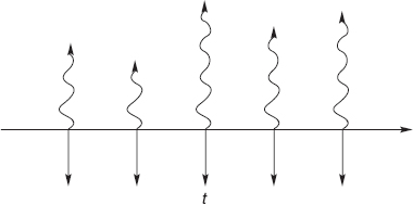
The first exchange of payments is made on 7th January 2008, six months after the deal is signed. How much money changes hands on that first date? We must pay 0.03 × $100,000,000 = $3,000,000. The cashflow in the opposite direction will be at six-month LIBOR, as quoted six months previously, i.e. at the initiation of the contract. This is a very important point. The LIBOR rate is set six months before it is paid, so that in the first exchange of payments the floating side is known. This makes the first exchange special.
The second exchange takes place on 7th July 2008. Again we must pay $3,000,000, but now we receive LIBOR, as quoted on 7th January 2008. Every six months there is an exchange of such payments, with the fixed leg always being known and the floating leg being known six months before it is paid. This continues until the last date, 7th July 2012.
Why is the floating leg set six months before it is paid? This ‘minor’ detail makes a large difference to the pricing of swaps, believe it or not. It is no coincidence that the time between payments is the same as the maturity of LIBOR that is used, six months in this example. This convention has grown up because of the meaning of LIBOR, it is the rate of interest on a fixed-term maturity, set now and paid at the end of the term. Each floating leg of the swap is like a single investment of the notional principal six months prior to the payment of the interest. Hold that thought, we return to this point in a couple of sections to show the simple relationship between a swap and bonds.
There is also the LIBOR in arrears swap in which the LIBOR rate paid on the swap date is the six-month rate set that day, not the rate set six months before.
Swaps were first created to exploit comparative advantage. This is when two companies who want to borrow money are quoted fixed and floating rates such that by exchanging payments between themselves they benefit, at the same time benefiting the intermediary who puts the deal together. Here’s an example.
Two companies A and B want to borrow $50MM, to be paid back in two years. They are quoted the interest rates for borrowing at fixed and floating rates shown in Table 15.1.
Note that both must pay a premium over LIBOR to cover risk of default, which is perceived to be greater for company B.
Ideally, company A wants to borrow at floating and B at fixed. If they each borrow directly then they pay the following:
The total interest they are paying is

Table 15.1 Borrowing rates for companies A and B.
| Fixed | Floating | |
| A | 7% | six-month LIBOR + 30 bps |
| B | 8.2% | six-month LIBOR + 100 bps |
Table 15.2 Borrowing rates with no swap involved.
| A | six-month LIBOR + 30 bps (floating) |
| B | 8.2% (fixed) |
If only they could get together they’d only be paying

That’s a saving of 0.5%.
Let’s suppose that A borrows fixed and B floating, even though that’s not what they want. Their total interest payments are six-month LIBOR plus 8%. Now let’s see what happens if we throw a swap into the pot.
* A is currently paying 7% and B six-month LIBOR plus 1 %. They enter into a swap in which A pays LIBOR to B and B pays 6.95% to A. They have swapped interest payments.
Looked at from A’s perspective they are paying 7% and LIBOR while receiving 6.95%, a net floating payment of LIBOR plus 5 bps. Not only is this floating, as A originally wanted, but it is 25 bps better than if they had borrowed directly at the floating rate. There’s still another 25 bps missing, and, of course, B gets this. B pays LIBOR plus 100 bps and also 6.95% to A while receiving LIBOR from A. This nets out at 7.95%, which is fixed, as required, and 25 bps less than the original deal.
Where did I get the 6.95% from? Let’s do the same calculation with ‘x’ instead of 6.95.
Go back to *. A is currently paying 7% and B six-month LIBOR plus 1%. They enter into a swap in which A pays LIBOR to B and B pays x% to A. They have swapped interest payments.
Looked at from A’s perspective they are paying 7% and LIBOR while receiving ‘x’%, a net floating payment of LIBOR plus 7 − x%. Now we want A to benefit by 25 bps over the original deal, this is half the 50 bps advantage. (I’ve just unilaterally decided to divide the advantage equally, 25 bps each.) So…

i.e.

Not only does A now get floating, as originally wanted, but it is 25 bps better than if they had borrowed directly at the floating rate. There’s still another 25 bps missing, and, of course, B gets this. B pays LIBOR plus 100 bps and also 6.95% to A while receiving LIBOR from A. This nets out at 7.95%, which is fixed, as required, and 25 bps less than the original deal.
In practice the two counterparties would deal through an intermediary who would take a piece of the action.
Although comparative advantage was the original reason for the growth of the swaps market, it is no longer the reason for the popularity of swaps. Swaps are now very vanilla products existing in many maturities and more liquid than simple bonds.
Given the ubiquity of swaps you would expect the comparative advantage argument to have been arbed away. This is true. However, the arbitrage still exists in special circumstances. For example, floating loans usually come with provision for reviewing the spread over LIBOR every few months. If the company has become less creditworthy between reviews the spread will be increased. This is difficult to model or anticipate and so is outside the no-arbitrage concept.
When the swap is first entered into it is usual for the deal to have no value to either party. This is done by a careful choice of the fixed rate of interest. In other words, the ‘present value,’ let us say, of the fixed side and the floating side both have the same value, netting out to zero. Consider the two extreme scenarios, very high fixed leg and very low fixed leg. If the fixed leg is very high the receiver of fixed has a contract with a high value. If the fixed leg is low the receiver has a contract that is worth a negative amount. Somewhere in between is a value that makes the deal valueless. The fixed leg of the swap is chosen for this to be the case.
Such a statement throws up many questions: How is the fixed leg decided upon? Why should both parties agree that the deal is valueless?
There are two ways to look at this. One way is to observe that a swap can be decomposed into a portfolio of bonds (as we see shortly) and so its value is not open to question if we are given the yield curve. However, in practice the calculation goes the other way. The swaps market is so liquid, at so many maturities, that it is the prices of swaps that drive the prices of bonds. The fixed leg of a par swap (having no value) is determined by the market.
The rates of interest in the fixed leg of a swap are quoted at various maturities. These rates make up the swap curve, see Figure 15.3.
There are two sides to a swap, the fixed-rate side and the floating-rate side. The fixed interest payments, since they are all known in terms of actual dollar amount, can be seen as the sum of zero-coupon bonds. If the fixed rate of interest is rs then the fixed payments add up to


This is the value today, time t, of all the fixed-rate payments. Here there are N payments, one at each Ti. Of course, this is multiplied by the notional principal, but assume that we have scaled this to one.
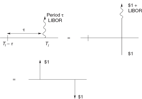
To see the simple relationship between the floating leg and zero-coupon bonds I draw some schematic diagrams and compare the cashflows. A single floating leg payment is shown in Figure 15.4. At time Ti there is payment of rτ of the notional principal, where rτ is the period τ rate of LIBOR, set at time Ti − τ. I add and subtract $1 at time Ti to get the second diagram. The first and the second diagrams obviously have the same present value. Now recall the precise definition of LIBOR. It is the interest rate paid on a fixed-term deposit. Thus the $1 + rτ at time Ti is the same as $1 at time Ti − τ. This gives the third diagram. It follows that the single floating rate payment is equivalent to two zero-coupon bonds. A single floating leg of a swap at time Ti is exactly equal to a deposit of $1 at time Ti − τ and a withdrawal of $1 at time τ.
Figure 15.4 A schematic diagram of a single floating leg in an interest rate swap and equivalent portfolios.
Now add up all the floating legs as shown in Figure 15.5, note the cancelation of all $1 (dashed) cashflows except for the first and last. This shows that the floating side of the swap has value
Figure 15.5 A schematic diagram of all the floating legs in a swap.


Bring the fixed and floating sides together to find that the value of the swap, to the receiver of the fixed side, is
This result is model independent. This relationship is independent of any mathematical model for bonds or swaps.
At the start of the swap contract the rate rs is usually chosen to give the contract par value, i.e. zero value initially. Thus
This is the quoted swap rate.
Swaps are now so liquid and exist for an enormous range of maturities that their prices determine the yield curve and not vice versa. In practice one is given rs(Ti) for many maturities Ti and one uses (15.1) to calculate the prices of zero-coupon bonds and thus the yield curve. For the first point on the discount-factor curve we must solve

i.e.
After finding the first j discount factors the j + 1th is found from

Figure 15.6 shows the forward curve derived from the data in Figure 15.3 by bootstrapping.
The above is a description of the vanilla interest rate swap. There any many features that can be added to the contract that make it more complicated, and most importantly, model dependent. A few of these features are mentioned here.
Callable and puttable swaps A callable or puttable swap allows one side or the other to close out the swap at some time before its natural maturity. If you are receiving fixed and the floating rate rises more than you had expected you would want to close the position. Mathematically we are in the early exercise world of American-style options. The problem is model dependent and is discussed in Chapter 18.
Extendible swaps The holder of an extendible swap can extend the maturity of a vanilla swap at the original swap rate.
Index amortizing rate swaps The principal in the vanilla swap is constant. In some swaps the principal declines with time according to a prescribed schedule. The index amortizing rate swap is more complicated still with the amortization depending on the level of some index, say LIBOR, at the time of the exchange of payments. We will see this contract in Chapter 18.
In the basis rate swap the floating legs of the swap are defined in terms of two distinct interest rates. For example, the prime rate versus LIBOR. A bank may have outstanding loans based on this prime rate but itself may have to borrow at LIBOR. It is thus exposed to basis risk and can be reduced with a suitable basis rate swap.
The basic equity swap is an agreement to exchange two payments, one being an agreed interest rate (either fixed or floating) and the other depending on an equity index. This equity component is usually measured by the total return on an index, both capital gains and dividend are included. The principal is not exchanged.
The equity basis swap is an exchange of payments based on two different indices.
A currency swap is an exchange of interest payments in one currency for payments in another currency. The interest rates can be both fixed, both floating or one of each. As well as the exchange of interest payments there is also an exchange of the principals (in two different currencies) at the beginning of the contract and at the end.
To value the fixed-to-fixed currency swap we need to calculate the present values of the cashflows in each currency. This is easily done, requiring the discount factors for the two currencies. Once this is done we can convert one present value to the other currency using the current spot exchange rate. If floating interest payments are involved we first decompose them into a portfolio of bonds (if possible) and value similarly.
The need and ability to be able to exchange one type of interest payment for another is fundamental to the running of many businesses. This has put swaps among the most liquid of financial contracts. This enormous liquidity makes swaps such an important product that one has to be very careful in their pricing. In fact, swaps are so liquid that you do not price them in any theoretical way, to do so would be highly dangerous. Instead they are almost treated like an ‘underlying’ asset. From the market’s view of the value we can back out, for example, the yield curve. We are helped in this by the fine detail of the swaps structure, the cashflows are precisely defined in a way that makes them exactly decomposable into zero-coupon bonds. And this can be done in a completely model-independent way. To finish this chapter I want to stress the importance of not using a model when a set of cashflows can be perfectly, statically and model-independently hedged by other cashflows. Any mispricing, via a model, no matter how small could expose you to large and risk-free losses.