© Springer Nature Switzerland AG 2020
E. Lindner et al. (eds.)Mathematical Modelling in Real Life ProblemsMathematics in Industry33https://doi.org/10.1007/978-3-030-50388-8_11

11. Optimising a Cascade of Hydro-Electric Power Stations

Marta Pascoal1, 2  
(1)
CMUC, Department of Mathematics, University of Coimbra, Coimbra, Portugal
(2)
Institute for Systems Engineering and Computers – Coimbra, Coimbra, Portugal
 
 
Marta Pascoal
Keywords
Hydroelectric power plantBranched cascadeOptimization

11.1 Introduction

Hydro electricity is electricity produced from hydropower and is responsible for a good share of the world’s total generated electricity. Most of this power comes from water stored in dams, usually coming from natural resources like rivers, rain or snow melts, which when released flows through a turbine activating a generator that produces electricity. The energy then produced depends on the volume of water that is released and the difference in height between the water starting and ending points. At times of less rain, or simply at high peak demands. there may be a shortage of water to turbine in the reservoirs, while electric power is still needed. To cope with such situations some power plants are capable of pumping water to higher reservoirs, which can be done when there is not enough water to be released when needed [2, 46].

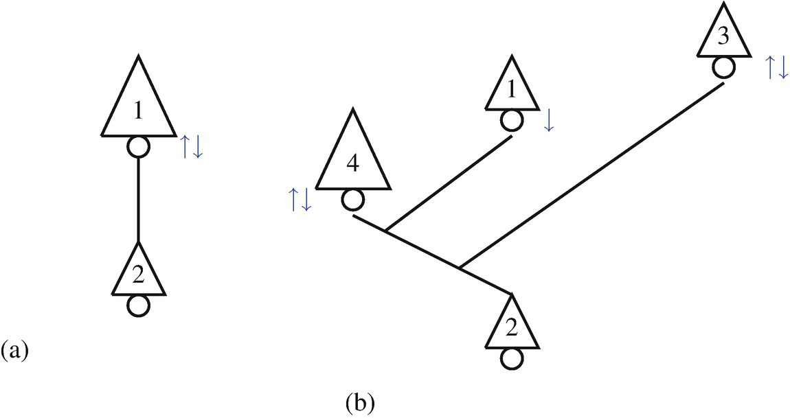
A cascade system of hydro-electric power stations is a set of stations connected as in a network where water flows between some of them. Two examples are shown in Fig. 11.1. The triangles and circles in the plots represent the hydro station reservoirs and turbines, respectively. The straight lines between the power stations show the connection between them, whereas the blue arrows attached to each circle define in which direction(s) each turbine is able to pump water.
../images/475466_1_En_11_Chapter/475466_1_En_11_Fig1_HTML.png
Fig. 11.1

Cascades with hydro-electric power stations. (a) Two hydro-electric power plants. (b) Four hydro-electric power plants

The purpose of this work is to model the operation of a branched cascade system like that depicted in Fig. 11.1b along 1 day, aiming at planning when each power station should release water downstream or pump it upstream. In this case, the turbines installed on hydro stations 3 and 4 have the ability of pumping water in both directions, that is, both from hydro stations 3 or 4 downstream to hydro station 2, as well as from hydro station 2 upstream to hydro stations 3 or 4. Such daily plan is decided based on a forecast for the energy market prices and with the goal of maximising the daily profit. The problem is modelled as a nonlinear optimisation problem, which can be solved using a mathematical programming environment like AMPL [3] or Matlab.

11.2 Problem Formulation

The problem of optimising the branched cascade of hydro electric power plants in Fig. 11.1b aims at planning the daily water flow in the cascade, with the goal of maximising the profit related with the electric power generation. This value depends on several features of the system, like the power that is consumed when the water is pumped upstream, the power that is generated by the hydro stations when water is released downstream, and, last but not least, on the energy market price oscillations. The main characteristics of that system are described in the following. To simplify we begin by considering the system with only two hydro stations, depicted in Fig. 11.1a.

11.2.1 Two Power Plants Cascade Model

We assume the water flow plan for the power plants is defined hourly for 1 day and first consider the simple cascade in Fig. 11.1a. Two sets of indices are used in the following, I = {1, 2}, which represents the set of power plants, and T = {1, 2, …, 24}, associated with the hours of the day.

Water Level, Water Head and Water Volume
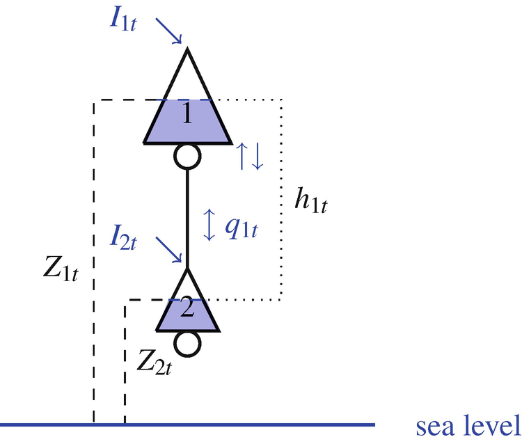
In order to characterise the system it is important to define the water level in each reservoir i with respect to the sea level, ξ, at instant t, denoted by Z it, for i ∈ I, t ∈ T, and depicted in Fig. 11.2. The difference between the water levels of two reservoirs is related with the power that is produced by releasing water from one reservoir to the next. These amounts are called the water head of reservoir i at moment t, and are denoted by h it and defined as

$$\displaystyle \begin{aligned} \begin{array}{ccl} h_{1t} & = & Z_{1t}-Z_{2t},\quad  t\in T\\ h_{2t} & = & Z_{2t}-\xi,\quad  t\in T \end{array}\end{aligned} $$
(11.1)
../images/475466_1_En_11_Chapter/475466_1_En_11_Fig2_HTML.png
Fig. 11.2

Cascade with two hydro-electric power plants

Additionally, the water levels vary according to the water volume in the reservoir, denoted by V it, for any i ∈ I and t ∈ T. Assuming that these quantities are known and that the reservoir has approximately the shape of a cone as in Fig. 11.3, Z it − Z i,t−1 can be estimated as the volume of a solid of revolution depending on a constant r related with the width of the reservoir,

$$\displaystyle \begin{aligned}V_{it}-V_{i,t-1}=\int_{Z_{i,t-1}}^{Z_{it}}\pi\,r^2y^2\,dy =\frac{\pi\,r^2}{3}\left(Z_{it}^3-Z_{i,t-1}^3\right),\end{aligned}$$
and, therefore,

$$\displaystyle \begin{aligned}Z_{it}=\sqrt[3]{Z_{i,t-1}^3+\frac{3}{\pi r^2}(V_{it}-V_{i,t-1})}.\end{aligned} $$
In practice, and to simplify the calculations, the water levels are usually updated as

$$\displaystyle \begin{aligned} Z_{it}=Z_i^0+\alpha_i(V_{it}-V_i^0)^{\beta_i},\quad  i\in I,\ t\in T\end{aligned} $$
(11.2)
with α i, β i given parameters, dependent on the shape and the characteristics of the reservoir, and 
$$Z_i^0$$
the nominal water level in the reservoir, i ∈ I. Finally, the values 
$$V_i^0$$
are given constants representing the nominal water volumes that correspond to 
$$Z_i^0$$
, for any i ∈ I [7].
../images/475466_1_En_11_Chapter/475466_1_En_11_Fig3_HTML.png
Fig. 11.3

Water reservoir

Limits are imposed to the minimum and the maximum amount of water that can be stored in each reservoir, either by using constraints over the volume of water, or over the level of water, in each of them. The constraints

$$\displaystyle \begin{aligned} Z_i^{\min}\le Z_{it}\le Z_i^{\max},\quad  i\in I, t\in T,\end{aligned} $$
(11.3)
model the latter situation, for 
$$Z_i^{\min }$$
, 
$$Z_i^{\max }$$
given constants, i ∈ I.
The Water Flow Rate
The volume of water in a reservoir i ∈ I is usually affected by inflows from natural resources, like rain, which are assumed to be estimated as I it, water from incoming discharges on upstream reservoirs, q jt, as well as water releases from the reservoir i itself to other downstream reservoirs, q it, i, j ∈ I, t ∈ T, as illustrated in Fig. 11.2. Thus,

$$\displaystyle \begin{aligned} \begin{array}{ccl} V_{1t} & = & V_{1,t-1}+I_{1t}-q_{1t},\quad  t\in T\\ V_{2t} & = & V_{2,t-1}+I_{2t}+q_{1t}-q_{2t},\quad  t\in T \end{array}\end{aligned} $$
(11.4)
are the flow conservation constraints needed to model the amount of water stored at any moment at reservoirs 1 and 2, respectively.
It is assumed that the flow rate q it is positive when the water is being pumped downstream, and negative if the water is being pumped upstream, i ∈ I, t ∈ T. Constraints that limit the flow rate at each reservoir are also necessary. In case of reservoirs that only pump water downstream (turbine) the bounds are

$$\displaystyle \begin{aligned} 0\le q_{it}\le q_i^0\sqrt{\frac{h_{it}}{h_i^0}},\quad  i\in I,\ t\in T\end{aligned} $$
(11.5)
and for the remaining reservoirs

$$\displaystyle \begin{aligned} \zeta_i\left(h_{it}-h_i^0\right)-q_i^0\le q_{it}\le q_i^0\sqrt{\frac{h_{it}}{h_i^0}},\quad  i\in I,\ t\in T \end{aligned} $$
(11.6)
Here, 
$$q_i^0$$
represents the nominal amount of turbined water in the reservoir i in the first case or the amount of nominal pumped water in the reservoir i in the second, ζ i is the pumping coefficient of the reservoir i, and 
$$h_i^0$$
is the nominal head of the reservoir i, i ∈ I [7].
Power and Revenue

The goal of the problem is to find a distribution of the times for each hydro plant to pump water downstream (called turbining) or to pump water upstream (called pumping up) along the day, in order to maximise the profit resulting from the produced power. The hourly prices of energy are denoted by P t and are assumed to be known, for t ∈ T. These values need to be combined with the electrical power that is produced and consumed by the power plants, which differs when water is only pumped downstream or when it can both be pumped downstream, thus producing power, and upstream, consuming it.

The power produced by the turbine of a hydroelectric station depends on the water flow, the height of the plant, the gravity acceleration, 9.8, and the equipment characteristics. A simple formula to model this quantity is

$$\displaystyle \begin{aligned}9.8q_{it}\mu_ih_{it},\end{aligned}$$
where μ i is a parameter specific to turbine i ∈ I that represents its efficiency in electricity production mode. In a more accurate model this value is also affected by an internal consumption factor ϕ i, which limits the net plant power output, as well as makes the power output grow slower as the water flow grows. The new model defines the power produced when turbining as

$$\displaystyle \begin{aligned}9.8q_{it}(h_{it}-\varDelta h_{it})\mu_i(1-\phi_i),\end{aligned}$$
where

$$\displaystyle \begin{aligned}\varDelta h_{it}=\varDelta h_i^0\left(\frac{q_{it}}{q_i^0}\right)^2\end{aligned}$$
represents friction losses when turbining or pumping, and 
$$\varDelta h_i^0$$
and 
$$q_i^0$$
are nominal values, i ∈ I.
At a given moment, each power plant either turbines water producing revenue, pumps it upstream with a certain cost in the short term, or the system is idle and there is zero flow. The formulae for the value of the power output and the price for pumping are combined as follows:

$$\displaystyle \begin{aligned} r_{it}=\left\{\begin{array}{cc} 9.8q_{it}(h_{it}-\varDelta h_{it}^T)\mu_i^T(1-\phi_i) & \mbox{ if } \; q_{it}\ge0\\ 9.8q_{it}(h_{it}+\varDelta h_{it}^P)\frac{1}{\mu_i^P(1-\phi_i)} & \mbox{ if } \; q_{it}<0 \end{array} \right.,\quad  i\in I,\ t\in T \end{aligned} $$
(11.7)
where

$$\displaystyle \begin{aligned}\varDelta h_{it}=\varDelta h_i^0 \left(\frac{q_{it}}{q_i^0}\right)^2\end{aligned}$$
represents friction losses when turbining (T) or pumping (P); both values expressed as a head loss. The nominal values 
$$\varDelta h_i^0$$
and 
$$q_i^0$$
are constants specific to each turbine; the parameters 
$$\mu _i^T$$
and 
$$1/\mu _i^P$$
represent efficiencies of turbines in electricity production mode and pumping mode, respectively. The objective function is then given by

$$\displaystyle \begin{aligned} \sum_{t\in T}P_t\sum_{i\in I}r_{it}, \end{aligned} $$
(11.8)
and the full formulation of the optimisation problem associated with the cascade depicted in Fig. 11.1a is

$$\displaystyle \begin{aligned} \begin{array}{llll} \text{maximise} & & \displaystyle\sum_{t\in T}P_t\sum_{i\in I}r_{it}\\ \text{subject to} & & h_{1t} = Z_{1t}-Z_{2t}, & t\in T\\ & & h_{2t} = Z_{2t}-\xi, & t\in T\\ & & Z_{it} = Z_i^0+\alpha_i(V_{it}-V_i^0)^{\beta_i}, & i\in I, \quad  t\in T\\ & & V_{1t} = V_{1,t-1}+I_{1t}-q_{1t}, & t\in T\\ & & V_{2t} = V_{2,t-1}+I_{2t}+q_{1t}-q_{2t}, & t\in T\\ & & Z_i^{\min} \le Z_{it} \le Z_i^{\max}, & i\in I, \quad  t\in T\\ & & 0 \le q_{2t} \le q_2^0\sqrt{\frac{h_{2t}}{h_2^0}}, & t\in T\\ & & \zeta_1\left(h_{1t}-h_1^0\right)-q_1^0 \le q_{1t} \le q_1^0\sqrt{\frac{h_{1t}}{h_1^0}}, & t\in T \end{array} \end{aligned} $$
(11.9)

11.2.2 Four Power Plants Cascade Model

The case of the four power plants cascade depicted in Fig. 11.1b can be seen as an extension of the previous one. In the following I = {1, 2, 3, 4} stands for the set of four hydro stations.

According to the presented scheme, in this case two turbines are able to work both in upstream and in downstream pumping modes, namely those located at the hydro electric plants 3 and 4. Thus, the previous flow conservation constraints are replaced by the conditions

$$\displaystyle \begin{aligned} \begin{array}{ccl} V_{2t} & = & V_{2,t-1}+I_{2t}+q_{1t}+q_{3t}+q_{4t}-q_{2t},\quad  t\in T\\ V_{it} & = & V_{i,t-1}+I_{it}-q_{it},\quad  i\in I-\{2\},\quad  t\in T \end{array} \end{aligned} $$
(11.10)
The formulation of the new optimisation model is as follows

$$\displaystyle \begin{aligned} \begin{array}{llll} \text{maximise} & & \displaystyle\sum_{t\in T}P_t\sum_{i\in I}r_{it}\\ \text{subject to} & & h_{it} = Z_{it}-Z_{2t}, & i\in I-\{2\}, \quad  t\in T\\ & & h_{2t} = Z_{2t}-\xi, & t\in T\\ & & Z_{it} = Z_i^0+\alpha_i(V_{it}-V_i^0)^{\beta_i} & i\in I,\quad  t\in T\\ & & V_{it} = V_{i,t-1}+I_{it}-q_{it}, & t\in T\\ & & V_{2t} = V_{2,t-1}+I_{2t}+q_{1t}+q_{3t}+q_{4t}-q_{2t}, & t\in T\\ & & Z_i^{\min}\le Z_{it}\le Z_i^{\max} & i\in I,\quad  t\in T\\ & & 0\le q_{it}\le q_i^0\sqrt{\frac{h_{it}}{h_i^0}} & i=1,2,\quad  t\in T\\ & & \zeta_i\left(h_{it}-h_i^0\right)-q_i^0\le q_{it}\le q_i^0\sqrt{\frac{h_{it}}{h_i^0}} & i=3,4,\quad  t\in T \end{array} \end{aligned} $$
(11.11)
It is noted that the variables q it are decision variables whereas V it, Z it and h it depend somehow on the flow rates q it, i ∈ I, t ∈ T. Like the formulation presented in the previous subsection, the problem that we want to solve (11.11), is a nonlinear optimisation problem. In fact, both the objective function in (11.8) and the sets of constraints (11.2), (11.5) and (11.6) are nonlinear.

11.3 Numerical Results

In [1] results of the implementation of the non-linear program (11.11) using the modelling language AMPL [3] are reported. Two cases were considered:
  1. 1.

    one where all the reservoirs started virtually empty, and

     
  2. 2.

    the other where all but the reservoir number 2 were empty and this one was almost full.

     
The input data of the model was provided by the company REN - Redes Energéticas, S.A.

The solution obtained for the first case had a small profit. Additionally, the increase/decrease in the flow rates followed the fluctuation in the energy prices, and pumping upstream appears in the optimal solution at times when the price is low, alternated by occasional pumping downstream when the price decreases. Usually the highest of the hydro plants is chosen as the sink of water pumped upstream.

The profit of the system was bigger in the second case and the optimal solution consisted mainly in pumping water downstream at maximum flow rate, as expected if no shortage of water occurs.

11.4 Concluding Remarks

The daily planning of a branched cascade of hydro power plants arranged as in Fig. 11.1b was modelled as a non-linear program. As concluding remarks it should be noted that it would be interesting in practice to extend the planning horizon to more than 1 day, and possibly include weekly patterns or seasonal characteristics. However, this will increase significantly the size of the problem. Also, this problem is associated with several natural phenomenon that are typically uncertain and, therefore, it would be most useful, and challenging, to handle it from a stochastic point of view.

Acknowledgements

This work was partially supported by the Centre for Mathematics of the University of Coimbra—UID/MAT/00324/2019 and by the Institute for Systems Engineering and Computers—Coimbra—UID/MULTI/00308/2019, funded by the Portuguese Government through FCT/MEC and co-funded by the European Regional Development Fund through the Partnership Agreement PT2020.